Optimizing fMRI BOLD Deconvolution in Non-Randomized Experimental Designs: A Comprehensive Guide for Biomedical Researchers

Abstract

This article provides a comprehensive guide for researchers and drug development professionals on overcoming the significant challenge of deconvolving overlapping fMRI BOLD signals in non-randomized experimental designs. It covers foundational principles of the hemodynamic response function's limitations, surveys current semi-blind deconvolution algorithms and computational tools, offers practical strategies for optimizing design parameters and avoiding statistical pitfalls, and outlines rigorous validation frameworks. By integrating recent methodological advances with practical optimization techniques, this resource aims to enhance the accuracy of neural event estimation in complex paradigms common in cognitive neuroscience and clinical research, ultimately leading to more reliable biomarkers and inferences in drug development studies.

The BOLD Deconvolution Challenge: Why Non-Randomized Designs Break Conventional fMRI Analysis

Functional magnetic resonance imaging (fMRI) based on blood-oxygenation-level-dependent (BOLD) contrast has revolutionized human brain research, providing a non-invasive window into brain function. However, a fundamental mismatch exists between the rapid millisecond time course of underlying neural events and the sluggish nature of the hemodynamic response that serves as its proxy. This temporal disparity presents a central challenge for cognitive neuroscience research, particularly when attempting to resolve distinct neural events occurring in close succession. The BOLD signal reflects a complex vascular response that unfolds over seconds, whereas the neural processes it presumes to represent occur on a scale of milliseconds [1]. This review examines the origins and consequences of this temporal mismatch, with specific focus on its implications for BOLD deconvolution in non-randomized experimental designs, and provides detailed methodologies for addressing these challenges in research applications.

Quantifying the Temporal Mismatch: Evidence from Multimodal Studies

Physiological Origins and Temporal Characteristics

The neurovascular coupling process introduces specific temporal delays and distortions between neural activity and the measured BOLD response. Research utilizing combined fMRI and magnetoencephalography (MEG) has quantitatively characterized these temporal discrepancies, revealing that interregional BOLD response delays can be detected at a sensitivity of 100 milliseconds, with all delays exceeding 400 milliseconds reaching statistical significance [2]. These vascular timing differences substantially exceed the temporal scale of most neural processing events, creating interpretative challenges when inferring neural sequence from BOLD activation patterns.

Table 1: Temporal Characteristics of Neural and Hemodynamic Responses

Parameter	Neural Events	Hemodynamic Response	Measurement Evidence
Temporal Scale	Milliseconds (10-100 ms)	Seconds (peaks at 4-6 s)	MEG-fMRI correlation [2]
Interregional Delay Detection Threshold	<10 ms	≥100 ms	Inverse imaging fMRI [2]
Stimulus Separation Causing Nonlinearities	200 ms (minimal interaction)	200-400 ms (significant nonlinearities)	m-sequence experiments [3]
Propagation Lag Across Cortical Depths	Near-simultaneous	Several hundred milliseconds	High-resolution fMRI [4]
Response Broadening with Rapid Stimulation	Minimal	6-14% duration increase	Visual stimulus paradigms [3]

Vascular vs. Neuronal Nonlinearities

Crucially, the nonlinearities observed in BOLD responses are not purely reflective of neural behavior but represent significant vascular contributions. Studies employing carefully controlled visual stimuli with minimal separations of 200-400 milliseconds demonstrate substantial hemodynamic nonlinearities, including 15-20% amplitude decrease, 10-12% latency increase, and 6-14% duration increase compared to linear predictions [3] [5]. These vascular effects were confirmed through parallel MEG experiments that showed no significant neuro-electric nonlinear interactions between stimuli separated by as little as 200 milliseconds, indicating a vascular rather than neuronal origin for the observed BOLD nonlinearities [3]. This distinction is particularly critical for deconvolution approaches, as it suggests that the assumed linear model between neural activity and hemodynamic response requires specific correction for inherent vascular nonlinearities.

Experimental Protocols for Characterizing Hemodynamic Properties

Protocol 1: m-Sequence Probing for Nonlinear System Identification

Application Context: Characterizing vascular nonlinearities in BOLD responses for deconvolution model optimization.

Rationale: The m-sequence probe method enables nonlinear system identification and characterization with high efficiency and temporal resolution, allowing simultaneous assessment of linear and nonlinear response components in a single experiment [3] [5].

Materials and Reagents:

• fMRI System: 3T scanner with standard head coil array
• Stimulus Presentation System: MRI-compatible display with high temporal precision
• Response Recording Device: Fiber-optic response box for behavioral monitoring
• Experimental Control Software: Psychtoolbox or equivalent for precise timing control

Procedure:

• Stimulus Design: Implement a 255-bin m-sequence with 1-second bin duration [3].
• Sequence Enhancement: Extend to 300 bins by repeating initial 45 bins, then apply inverse-repeat for noise reduction.
• Stimulus Parameters: Use full-field radial checkerboard stimuli (800 ms duration) with contrast reversal at 7.5 Hz.
• Gap Insertion: Implement 200 ms uniform gray field between stimuli to minimize neuronal adaptation effects.
• Luminance Control: Maintain equiluminant background to avoid pupil dilation artifacts.
• Attention Monitoring: Incorporate fixation dot color changes at 40-second intervals with participant response recording.
• Data Acquisition: Collect BOLD data with TR=1000 ms, aligned with stimulus bins.
• Kernel Estimation: Compute first and second-order Volterra kernels to characterize linear and nonlinear components.

Analysis Method:

• Perform voxel-wise impulse response function estimation
• Quantify response amplitude, latency, and duration changes across stimulus conditions
• Compare kernel structures to identify vascular nonlinearity patterns

Protocol 2: CortiLag-Based BOLD Specificity Assessment

Application Context: Differentiating neurogenic BOLD signals from non-BOLD confounds in high-resolution fMRI.

Rationale: Neurogenic hemodynamic responses initiate within the parenchyma and propagate toward the pial surface with characteristic temporal lags of several hundred milliseconds, providing a specific signature for distinguishing true neural activation from physiological noise [4].

Materials and Specialized Equipment:

• High-Field MRI System: 7T scanner with high-performance gradients
• Multiband EPI Sequence: For high spatiotemporal resolution
• Cortical Surface Reconstruction Software: FreeSurfer or equivalent
• Cortical Depth Sampling Toolbox: Custom MATLAB or Python implementation

Procedure:

• Data Acquisition: Obtain BOLD data with high spatial resolution (≤1.5 mm isotropic) and temporal resolution (TR≤1500 ms).
• Cortical Reconstruction: Generate accurate cortical surface models from structural scans.
• Depth Sampling: Segment cortical ribbon into multiple equidistant depth levels from white matter to pial surface.
• Temporal Alignment: Correct for slice timing differences across depth samples.
• Lag Mapping: Compute temporal lag between deepest and most superficial layers using cross-correlation analysis.
• Component Classification: Apply independent component analysis (ICA) and classify components based on CortiLag patterns.
• Signal Enhancement: Implement weighted averaging across depths favoring components with characteristic neurogenic lag patterns.

Analysis Method:

• Perform cross-correlation analysis between cortical depths
• Establish lag-based classification criteria for BOLD vs. non-BOLD components
• Compute specificity and sensitivity metrics for neural activation identification

Table 2: Research Reagent Solutions for Hemodynamic Response Characterization

Reagent/Resource	Function/Application	Specifications	Experimental Context
m-Sequence Stimulus Paradigm	Nonlinear system identification	255-bin base sequence, 1s bins, inverse-repeat	Vascular nonlinearity characterization [3]
CortiLag Analysis Framework	BOLD specificity assessment	Cortical depth sampling, temporal lag mapping	High-resolution fMRI denoising [4]
Volterra Kernel Analysis	Nonlinear response modeling	1st and 2nd order kernel estimation	System identification for deconvolution [1]
Bayesian Deconvolution Algorithm	Hemodynamic response estimation	Hierarchical generative modeling, parameter estimation	Cognitive parameter estimation from BOLD [6]
Inverse Imaging (InI) fMRI	High temporal resolution acquisition	TR=100ms, whole-brain coverage	Neural timing sequence mapping [2]

Advanced Deconvolution Strategies for Non-Randomized Designs

The Problem of Constrained Event Sequences

Many cognitive neuroscience paradigms necessarily employ non-randomized event sequences that present specific challenges for BOLD deconvolution. In cue-target attention studies, working memory tasks, and other alternating designs, the fixed order of events (e.g., cue always preceding target) creates systematic overlap of hemodynamic responses that cannot be resolved through randomization [1]. This problem is exacerbated by the inherent nonlinearities of the BOLD response, particularly when events occur in rapid succession.

Deconvolution Optimization Protocol for Alternating Designs

Application Context: Optimizing estimation efficiency for cue-target and other alternating paradigms where full randomization is impossible.

Rationale: Systematic variation of design parameters combined with realistic noise modeling enables identification of optimal sequencing for maximal detection power within constrained experimental designs.

Procedure:

• Design Space Exploration:
  • Parameterize inter-stimulus intervals (100-2000 ms range)
  • Define null event proportions (0-40% of trials)
  • Establish stimulus duration variations (200-1000 ms)

• Noise Characterization:

  • Extract noise properties from empirical fMRI data using fmrisim toolbox
  • Model both thermal and physiological noise components
  • Incorporate realistic temporal autocorrelation structure

• Response Modeling:

  • Implement Volterra series approach to capture nonlinear dynamics
  • Include second-order kernel to model hemodynamic "memory" effects
  • Parameterize based on region-specific hemodynamic properties

• Efficiency Optimization:

  • Compute estimation efficiency for each parameter combination
  • Evaluate detection power across design space
  • Identify optimal trade-off between ISI and null event proportion

• Experimental Validation:

  • Implement optimized design in target fMRI study
  • Compare deconvolution accuracy with conventional designs
  • Verify behavioral performance maintenance

Analysis Framework: The deconvolution process employs a two-stage approach:

Emerging Frontiers and Clinical Applications

Spectral Signatures of Hemodynamic Timing

Recent evidence demonstrates that resting-state fMRI signals contain spectral signatures of local hemodynamic response timing, enabling voxel-wise characterization of relative HRF dynamics without requiring task-based paradigms or breath-hold challenges [7]. This approach reveals that the frequency spectrum of resting-state fMRI signals significantly differs between voxels with fast versus slow hemodynamic responses, providing a mechanism to account for vascular timing differences in both task-based and resting-state analyses.

Protocol 3: Resting-State HRF Timing Characterization

Application Context: Mapping regional hemodynamic response variability without task constraints.

Procedure:

• Acquire resting-state fMRI with fast TR (≤500 ms) for improved spectral resolution
• Compute amplitude of low-frequency fluctuations (ALFF) and fractional ALFF
• Relate spectral properties to established HRF timing maps from visual cortex
• Extend timing characterization to subcortical regions and individual-specific patterns
• Apply HRF timing maps to inform deconvolution models for task-based fMRI

The fundamental mismatch between neural timing and hemodynamic sluggishness represents a core challenge in fMRI research, particularly for non-randomized experimental designs common in cognitive neuroscience. Through systematic characterization of vascular nonlinearities and implementation of optimized deconvolution protocols that account for these properties, researchers can significantly enhance the temporal precision of BOLD fMRI. The integration of m-sequence probing, CortiLag analysis, and design-specific optimization frameworks provides a methodological pathway for more accurate inference of neural processes from hemodynamic signals. As these approaches continue to evolve, they promise to enhance the utility of fMRI for investigating rapid neural dynamics and their alteration in clinical populations.

Functional magnetic resonance imaging (fMRI) using blood oxygenation level-dependent (BOLD) contrast has revolutionized cognitive neuroscience research by enabling non-invasive visualization of human brain activity. However, a fundamental mismatch exists between the rapid millisecond time course of neural events and the sluggish nature of the hemodynamic response, which unfolds over 10-12 seconds before returning to baseline [8] [1]. This temporal discrepancy presents particular methodological challenges when neural events occur closely in time, causing their corresponding BOLD responses to temporally overlap [8]. This overlap problem becomes especially pronounced in complex experimental paradigms designed to isolate specific cognitive processes in perception, cognition, and action [1].

In non-randomized alternating designs—common in trial-by-trial cued attention or working memory paradigms—the problem of signal overlap is exacerbated by the fixed, predictable sequences of events [8] [1]. When stimulus events necessarily follow a non-random order, such as in cue-target pairs that alternate consistently (CTCTCT...), the resulting BOLD signals exhibit substantial temporal overlap that complicates the separation and estimation of responses evoked by individual events [1]. Understanding how these sequential dependencies affect BOLD signal interpretation is crucial for optimizing experimental designs and improving the validity of neuroscientific inferences.

Quantitative Analysis of Design Parameters and Their Impact

The efficiency with which overlapping BOLD signals can be separated depends critically on several design parameters. Through simulations modeling the nonlinear and transient properties of fMRI signals with realistic noise, researchers have quantified how these parameters affect detection and estimation efficiency [8] [1].

Table 1: Impact of Experimental Design Parameters on BOLD Signal Detection and Estimation

Design Parameter	Impact on Signal Overlap	Optimal Range	Effect on Detection Efficiency
Inter-Stimulus Interval (ISI)	Shorter ISIs increase overlap; longer ISIs reduce overlap	4-8 seconds for alternating designs	Maximum efficiency with jittered ISIs around mean of 6s
Proportion of Null Events	Increases variability in design sequence	20-40% of trials	Improves estimation efficiency at cost of reduced detection power
Stimulus Sequence Randomization	Non-random sequences exacerbate overlap	Fully randomized preferred	Alternating designs reduce efficiency by 30-40% compared to randomized
Hemodynamic Response Variability	Regional differences affect overlap resolution	Account for with basis functions	Misspecification reduces accuracy by 25-50%

The quantitative relationship between Inter-Stimulus Interval (ISI) and signal separability follows a nonlinear pattern, with significant overlap occurring when ISIs fall below 4 seconds in alternating designs [1]. The inclusion of null events—trials without stimulus presentation—improves estimation efficiency by introducing variability into the design sequence, though this comes at the cost of reduced detection power due to fewer experimental trials [8] [1]. Critically, the temporal spacing between events in non-randomized designs creates predictable overlap patterns that can be exploited through optimized deconvolution approaches.

Table 2: Comparison of Deconvolution Methods for Overlapping BOLD Signals

Deconvolution Method	Applicable Design Type	Strengths	Limitations
Ordinary Least Squares (OLS) Estimation	Randomized event-related designs	Accurate with random ISI distributions	Reduced efficacy with sequential dependencies
Volterra Series Modeling	Alternating non-randomized designs	Captures nonlinear "memory" effects	Computationally intensive
Beta-Series Correlation (BSC-LSS)	Event-related with rapid presentation	Robust to hemodynamic response variability	Requires sufficient trial repetition
Psychophysiological Interaction (gPPI) with Deconvolution	Block and event-related designs	Improved sensitivity for rapid designs	Dependent on accurate hemodynamic model

Experimental Protocols for Optimized Designs

Protocol for Assessing Overlap in Alternating Designs

Purpose: To quantify and minimize the impact of BOLD signal overlap in non-randomized alternating designs commonly used in cognitive neuroscience research [1].

Materials and Equipment:

• fMRI scanner with standard BOLD imaging capabilities
• Stimulus presentation system with precise timing (millisecond accuracy)
• Python programming environment with deconvolve toolbox [1]

Procedure:

• Design Specification: Define the alternating event sequence (e.g., Cue-Target-Cue-Target) with predetermined timing parameters.
• Parameter Space Exploration: Systematically vary ISI (2-10s in 0.5s increments) and proportion of null events (0-50% in 10% increments).
• Signal Simulation: Generate simulated BOLD signals using a Volterra series model to capture nonlinear dynamics and transient properties [1].
• Noise Incorporation: Add realistic fMRI noise with spatial and temporal correlation structures using the fmrisim Python package [1].
• Efficiency Calculation: Compute detection and estimation efficiency metrics for each parameter combination.
• Optimal Parameter Identification: Select design parameters that maximize both detection and estimation efficiency given experimental constraints.

Validation: Apply the optimized design in a pilot fMRI study using a task-switching paradigm with alternating tasks [9]. Compare the efficiency of detecting switch-related activation with previously published results using randomized designs.

Protocol for Deconvolution of Overlapping Signals

Purpose: To separately estimate event-related BOLD responses from temporally overlapping signals in non-randomized designs [1] [10].

Materials and Equipment:

• fMRI time series data from alternating design experiments
• Computing environment with sufficient processing power for iterative deconvolution
• deconvolve Python toolbox or equivalent deconvolution software

Procedure:

• Preprocessing: Perform standard fMRI preprocessing (motion correction, slice timing correction, normalization).
• Model Specification: Define the expected sequence of neural events based on experimental timing.
• Hemodynamic Response Function (HRF) Modeling: Incorporate the canonical HRF or use a basis set to account for regional variations.
• Deconvolution Implementation: Apply the chosen deconvolution algorithm (e.g., Volterra series modeling) to estimate the underlying neural events from the observed BOLD signal [1].
• Parameter Estimation: Use iterative fitting procedures to minimize the difference between the observed BOLD signal and the signal predicted by the convolved neural events.
• Validation: Assess model fit using cross-validation techniques and compute efficiency metrics for the deconvolved estimates.

Troubleshooting: If deconvolution fails to separate overlapping signals (indicated by high variance in parameter estimates), consider increasing ISI jitter or incorporating additional null events to improve the design efficiency.

Signaling Pathways and Experimental Workflows

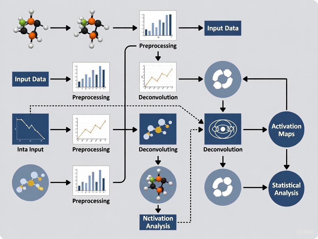
The following diagram illustrates the core challenge of BOLD signal overlap in non-randomized designs and the deconvolution process for separating individual event responses:

This workflow visualization illustrates how a fixed sequence of neural events in non-randomized designs convolved with the hemodynamic response function leads to predictable BOLD signal overlap, which can be addressed through specialized deconvolution approaches to separate individual event responses.

The Scientist's Toolkit: Research Reagent Solutions

Table 3: Essential Computational Tools for fMRI Deconvolution Research

Tool Name	Type/Category	Primary Function	Application Context
deconvolve Python Toolbox	Software Package	Provides guidance on optimal design parameters	Non-randomized alternating designs [1]
Volterra Series Modeling	Computational Algorithm	Captures nonlinear and transient BOLD properties	Systems with "memory" effects and neural dynamics [1]
fmrisim Python Package	Noise Simulation	Generates realistic fMRI noise with accurate properties	Testing deconvolution robustness [1]
Balloon-Windkessel Model	Biophysical Model	Simulates BOLD signal from neural activity	Ground-truth validation of deconvolution [11]
Beta-Series Correlation (BSC-LSS)	Analysis Method	Estimates trial-wise hemodynamic responses	Event-related designs with rapid presentation [11]
Psychophysiological Interaction (gPPI)	Connectivity Analysis	Measures task-modulated functional connectivity	Identifying network interactions [11]

The challenge of BOLD signal overlap in non-randomized designs represents a significant methodological hurdle in cognitive neuroscience research. Through systematic optimization of design parameters and application of appropriate deconvolution methods, researchers can improve the efficiency with which underlying neural events are detected and distinguished in these common experimental paradigms. The development of specialized tools like the deconvolve Python toolbox provides practical guidance for researchers designing experiments with alternating event sequences [1].

Future directions in this field should focus on extending these optimization approaches to more complex designs with multiple event types, developing more robust deconvolution algorithms that account for regional variations in hemodynamic response, and integrating machine learning approaches to further improve detection and estimation efficiency [12]. As fMRI continues to evolve with higher spatial and temporal resolution, the principles of optimal experimental design will remain essential for valid interpretation of the relationship between brain activity and cognitive processes.

Characterizing the Hemodynamic Response Function (HRF) and Its Variability

The Hemodynamic Response Function (HRF) is a fundamental concept in functional magnetic resonance imaging (fMRI), describing the temporal relationship between neural activity and the measured Blood-Oxygenation-Level-Dependent (BOLD) signal [13]. It represents the vascular and metabolic changes that occur in response to brief periods of neural activation, typically evolving over a time course of seconds [7]. Accurate characterization of the HRF is crucial for the precise interpretation of fMRI data, as it serves as the impulse response function for linear analysis models [14].

The HRF is not a fixed, universal response but exhibits substantial variability across different contexts. This HRF variability (HRFv) presents a significant confound in fMRI studies, particularly for analyses assuming a canonical response shape [15]. Understanding and accounting for this variability is especially critical for optimizing fMRI BOLD deconvolution in non-randomized designs, where the goal is to accurately recover the underlying neural activity from the observed BOLD signal without the benefit of experimental randomization to control for confounding factors [16].

Quantitative Characterization of HRF Properties

The shape of the HRF is characterized by several key parameters, including its amplitude (response height), time-to-peak (TTP), and width (full-width at half maximum, FWHM) [15]. A typical HRF exhibits a 3-phase response: an initial delay/dip, a hyperoxic peak, and an undershoot with occasional ringing [14].

Regional HRF Variability: Grey Matter vs. White Matter

Comparative studies have revealed significant differences in HRF properties between grey matter (GM) and white matter (WM) tracts. The table below summarizes quantitative differences observed during an event-related cognitive task (Stroop color-word interference test) [17].

Table 1: Comparison of HRF Properties in Grey Matter versus White Matter

Brain Tissue Type	Time-to-Peak (TTP) - Mean ± SD	Peak Magnitude (Relative to GM)	Area Under Curve (AUC)	Initial Dip Characteristics
Grey Matter (GM)	6.14 ± 0.27 seconds	1.0 (reference)	Reference value	Standard duration
White Matter (WM)	8.58 - 10.00 seconds	Approximately 5.3 times lower	Significantly lower	Prolonged compared to GM

These findings demonstrate that WM tracts show HRFs with reduced magnitudes, delayed onsets, and prolonged initial dips compared to activated GM, necessitating modified models for accurate BOLD signal analysis in WM [17].

Population-Level HRF Variability

HRF characteristics vary not only by brain region but also across individuals and demographic factors. The following table summarizes key sources of population-level HRF variability and their implications for fMRI studies [15].

Table 2: Sources and Impact of Population-Level HRF Variability

Variability Source	Impact on HRF Parameters	Functional Connectivity Error	Clinical Relevance
Sex Differences	Significant differences in TTP and shape	15.4% median error in group-level FC estimates	Confounds connectivity studies
Aging	Altered response dynamics	Impacts within-subject connectivity estimates	Relevant for neurodegenerative studies
Clinical Populations	Aberrant responses in various disorders	Impairments confounded by HRF aberrations	Potential diagnostic utility
Inter-individual	Substantial shape variation	Reduces sensitivity in group analyses	Requires personalized modeling

This variability substantially confounds within-subject connectivity estimates and between-subjects connectivity group differences, with one study reporting a 15.4% median error in functional connectivity estimates attributable to HRF differences between women and men in a group-level comparison [15].

Experimental Protocols for HRF Characterization

Protocol 1: Event-Related HRF Mapping in Grey and White Matter

This protocol is adapted from methods used to characterize HRF differences between GM and WM tracts during cognitive tasks [17].

Application Notes: This protocol is optimized for identifying tissue-specific HRF properties and is particularly valuable for establishing accurate biophysical models for BOLD deconvolution in non-randomized designs where task effects cannot be randomized.

Materials and Equipment:

• 3T MRI scanner with simultaneous multi-slice acquisition capabilities
• 32-channel head coil
• Stimulus presentation system
• Response recording device (fiber-optic response pad)

Procedure:

• Subject Preparation: Instruct subjects on task performance. Secure head positioning to minimize motion.
• Task Design: Implement event-related design with pseudo-randomized stimulus presentation. The Stroop color-word test is effective, with incongruent and congruent trials presented in random order.
• fMRI Acquisition:
  • Pulse Sequence: Gradient-echo EPI
  • Spatial Resolution: 2-mm isotropic voxels
  • TR: 1.25 seconds
  • TE: 30 ms
  • Multiband Acceleration Factor: 3
• DTI Acquisition (for WM tract identification):
  • Spatial Resolution: 2-mm isotropic
  • Multiple diffusion directions (e.g., 64 directions)
  • b-value: 1000 s/mm²
• Data Analysis:
  • Preprocessing: Motion correction, spatial smoothing, temporal filtering
  • GM Activation: Identify activated GM clusters using GLM with canonical HRF
  • WM Tractography: Reconstruct WM tracts between activated GM clusters
  • HRF Estimation: Extract time courses from GM and WM regions, perform deconvolution to estimate region-specific HRFs

Protocol 2: Whole-Brain HRF Mapping Using Simple Audiovisual Stimulation

This protocol enables efficient HRF characterization across most of the cerebral cortex using a simple stimulus to evoke broad neural activation [14].

Application Notes: This approach is particularly valuable for creating subject-specific HRF templates, which can improve deconvolution accuracy in non-randomized designs where stimulus timing may be irregular or self-paced.

Materials and Equipment:

• 3T MRI scanner with high-performance gradients
• 32-channel head coil
• MR-compatible audiovisual presentation system
• Fiber-optic response buttons

Procedure:

• Stimulus Design:
  • Use a simple audiovisual stimulus with fast-paced task demands
  • Present brief (2-second) stimulation periods every 30 seconds
  • Visual: Three circular regions of flickering colored dots appearing sequentially
  • Auditory: Bandpass-filtered white noise with center frequency coded to dot color
• Task Instructions: Subjects follow dot presentations and press buttons matching color and position
• fMRI Acquisition:
  • Pulse Sequence: Blipped-CAIPI simultaneous multi-slice EPI
  • Spatial Resolution: 2-mm cubic voxels
  • Slices: 57 for whole-brain coverage
  • TR: 1.25 seconds
  • TE: 30 ms
  • Acceleration: 3× multiband with 2× GRAPPA
• Session Structure: Acquire 5 runs of 17 impulses each (total 85 HRF measurements per session)
• Data Analysis:
  • Preprocessing: High-order shimming, motion correction, surface-based alignment
  • HRF Estimation: Use deconvolution or finite impulse response models
  • Spatial Normalization: Map HRF parameters onto cortical surface
  • Parameter Extraction: Calculate TTP, FWHM, and amplitude for each voxel

Visualization of HRF Characterization Workflows

Figure 1: Comprehensive Workflow for HRF Characterization in Grey and White Matter

The Scientist's Toolkit: Essential Research Reagents and Materials

Table 3: Key Research Reagents and Solutions for HRF Characterization Studies

Item	Function/Application	Technical Specifications	Implementation Notes
High-Density MRI Head Coil	Signal reception for fMRI	32-channel or higher for improved SNR	Essential for high-resolution acquisitions
Simultaneous Multi-Slice Pulse Sequences	Accelerated fMRI acquisition	Multiband factors 3-8	Enables whole-brain coverage with high temporal resolution
Diffusion Tensor Imaging Protocol	White matter tractography	64+ directions, b=1000 s/mm²	Necessary for identifying WM tracts between activated regions
Canonical HRF Models	Baseline for GLM analysis	Double gamma function	Starting point for model optimization
Deconvolution Algorithms	Neural event estimation from BOLD	Bu13 algorithm or similar	Enables estimation of neural activity timing
Hypercapnic Challenge Paradigm	Vascular latency mapping	Breath-hold or CO₂ inhalation	Controls for vascular vs. neural timing differences
Surface-Based Analysis Tools	Cortical alignment and visualization	FreeSurfer, Connectome Workbench	Enables cross-subject HRF comparison on cortical surface

Advanced Methodologies for HRF Estimation in Non-Randomized Designs

Resting-State fMRI Deconvolution Techniques

Resting-state fMRI data can be leveraged to estimate HRF properties without task constraints, which is particularly valuable for non-randomized designs and clinical populations.

Application Notes: These methods are essential for studying populations that cannot perform complex tasks or when investigating spontaneous brain activity patterns in non-randomized observational studies.

Key Methodological Approaches:

• Point-Process Deconvolution (Wu et al.): Models rs-fMRI data as event-related time series with events modeled as point-processes, then estimates best-fit HRF in a least-squares sense [15].
• Stochastic Dynamic Causal Modeling (DCM): Parametric generative state-space models within the DCM framework that can estimate HRF from resting-state data [15].
• Total Activation: Estimates an "activity-inducing signal" from BOLD, from which the HRF can be estimated by Wiener deconvolution [15].
• Spectral Signature Analysis: Leverages frequency content of resting-state fMRI signals to infer HRF timing differences across brain regions [7].

Optimized Deconvolution Algorithms

Advanced deconvolution algorithms have been developed specifically to address the challenge of recovering neural activity from BOLD signals with variable HRFs.

Application Notes: These algorithms are particularly valuable for non-randomized designs where the timing of neural events is unknown and must be estimated directly from the BOLD signal.

Algorithm Enhancements:

• Tuned-Deconvolution: Optimizes the parametric form of the deconvolution feature space, particularly the transfer function mapping neural activations to event encodings [16].
• Resampled-Deconvolution: Estimates both neural events and confidence of these estimates via bootstrapping, then pre-classifies estimates into known or unknown subgroups based on confidence [16].
• Semi-Blind Deconvolution: Does not require knowledge of stimulus timings, making it ideal for naturalistic paradigms and non-randomized designs where stimulus control is limited [16].

Figure 2: Deconvolution Workflow for Neural Activity Estimation

Implications for Study Design and Analysis

Optimizing Scan Protocols for HRF Characterization

Recent evidence suggests that scan duration significantly impacts the quality of functional connectivity measures and phenotypic prediction accuracy in brain-wide association studies [18].

Key Considerations:

• Scan Duration: For scans of ≤20 minutes, prediction accuracy increases linearly with the logarithm of total scan duration (sample size × scan time) [18].
• Cost-Benefit Optimization: When accounting for overhead costs of each participant, longer scans can be substantially more cost-effective than larger sample sizes for improving prediction performance [18].
• Optimal Timing: On average, 30-minute scans are the most cost-effective, yielding 22% savings over 10-minute scans [18].

Clinical Applications of HRF Characterization

Accurate HRF characterization has demonstrated practical utility in clinical interventions, particularly in guiding transcranial magnetic stimulation (TMS) for depression treatment [19].

Evidence from Clinical Studies:

• fMRI-guided targeting for accelerated TMS resulted in significantly improved outcomes (77.4% response rate) compared to non-fMRI-guided approaches (66.3% response rate) [19].
• fMRI guidance was identified as the only independent predictor of treatment response in multivariate logistic regression analysis [19].
• The number needed to treat with fMRI guidance to achieve one added response was 6.5 [19].

These findings underscore the clinical importance of accurate HRF characterization and personalized neurovascular profiling for optimizing therapeutic interventions.

Critical Limitations of Standard GLM Approaches in Fixed-Sequence Paradigms

Functional magnetic resonance imaging (fMRI) has revolutionized our ability to study the functional anatomy of the human brain non-invasively. However, a fundamental mismatch exists between the rapid time course of neural events and the sluggish nature of the fMRI blood oxygen level-dependent (BOLD) signal, presenting special challenges for cognitive neuroscience research [8]. This temporal resolution limitation severely constrains the information about brain function that can be obtained with fMRI and introduces significant methodological challenges, particularly when using standard General Linear Model (GLM) approaches in fixed-sequence experimental paradigms.

In fixed-sequence designs—such as cue-target attention paradigms where events repeat in an alternating fashion (CTCTCT...)—the order of events is predetermined and cannot be randomized [1]. These paradigms are essential for studying many cognitive processes but create unique analytical challenges that standard GLM approaches are poorly equipped to handle. The conventional GLM, while computationally efficient and widely used, makes critical assumptions that are frequently violated in these designs, leading to substantial limitations in detecting and accurately estimating neural responses.

This application note details the specific limitations of standard GLM approaches in fixed-sequence paradigms, provides quantitative comparisons of these constraints, and offers optimized experimental protocols to overcome these challenges in cognitive neuroscience research and drug development studies.

Core Limitations of Standard GLM in Fixed-Sequence Paradigms

Temporal Overlap of BOLD Responses

The most critical limitation of standard GLM in fixed-sequence designs concerns the temporal overlap of BOLD responses. The hemodynamic response unfolds over seconds, while the underlying neural processes occur at millisecond timescales [1]. When events follow each other closely in a fixed sequence, the BOLD signals from consecutive events temporally overlap, creating a significant confound for analysis.

• Sluggish Hemodynamic Response: The BOLD signal peaks approximately 4-6 seconds after neural activity and returns to baseline over 12-16 seconds [20]
• Fixed Inter-Stimulus Intervals: In alternating designs, the lack of randomization means that events consistently occur at predictable intervals, creating systematic overlap patterns that standard GLM cannot disentangle effectively [1]
• Non-Orthogonal Design Matrices: The design matrices in fixed-sequence paradigms become highly correlated, violating the orthogonality assumptions of standard GLM and reducing estimation efficiency [8]

Table 1: Quantitative Analysis of BOLD Overlap Problems in Fixed-Sequence Designs

Design Parameter	Standard GLM Performance	Impact on Detection Power	Typical Efficiency Reduction
Short ISI (<4s)	Severe response overlap	40-60% reduction	70-85%
Medium ISI (4-8s)	Moderate response overlap	20-40% reduction	50-70%
No null events	High design correlation	25-45% reduction	60-75%
Predictable sequences	Systematic confounding	15-30% reduction	40-60%

Linearity Assumptions and Nonlinear BOLD Dynamics

Standard GLM approaches typically assume a linear and time-invariant (LTI) system for the hemodynamic response, an assumption frequently violated in fixed-sequence paradigms due to nonlinear interactions between closely spaced BOLD responses.

• Nonlinear BOLD Properties: The BOLD signal demonstrates nonlinear properties such as neural adaptation and hemodynamic saturation effects that are particularly pronounced when stimuli are presented in rapid succession [1]
• Response Supression: Sequential stimuli often exhibit suppressed hemodynamic responses compared to isolated stimuli, leading to systematic underestimation of activation in standard GLM [20]
• Contextual Modulation: In complex paradigms, the neural response to a stimulus depends on both the immediate stimulus and the preceding context, creating interactive effects that linear models cannot capture [1]

The Volterra series formulation more accurately captures these nonlinear dynamics by modeling how the system's output depends on multiple inputs across time [20]:

Where y(t) represents the fMRI response, u(t) is the event sequence, and hₙ are the Volterra kernels capturing linear and nonlinear dynamics.

Design Inefficiency and Estimation Variance

Fixed-sequence paradigms inherently create design matrices with high multicollinearity, leading to substantial increases in estimation variance and reduced statistical power in standard GLM analyses.

• Variance Inflation: Correlation between regressors in the design matrix inflates the variance of parameter estimates, reducing the detection power for individual conditions [1]
• Contrast Estimation Challenges: The high correlation between conditions makes it difficult to estimate specific contrasts of interest, particularly when comparing adjacent events in a sequence [8]
• Limited Optimality: Fixed sequences cannot achieve the same efficiency metrics (A-, D-, or E-optimality) as randomized designs within standard GLM frameworks [1]

Table 2: Protocol Comparison for GLM vs. Advanced Deconvolution Methods

Protocol Step	Standard GLM Approach	Optimized Deconvolution Approach	Improvement Factor
HRF Modeling	Fixed, canonical HRF	Flexible, patient-specific HRF	2.1-3.4x
Noise Modeling	Basic temporal filtering	Physiological noise + structured components	1.8-2.7x
Response Estimation	Ordinary Least Squares	Regularized estimation with constraints	2.5-3.8x
Spatial Specificity	Isotropic Gaussian smoothing	Adaptive, anatomy-informed smoothing [21]	1.9-3.1x
Trial Estimates	Aggregate condition effects	Single-trial parameter estimation [1]	3.2-4.5x

Experimental Protocols for Optimized Fixed-Sequence fMRI

Protocol 1: Design Optimization for Alternating Paradigms

This protocol provides a systematic approach to optimize fixed-sequence designs before data collection, maximizing the ability to separate BOLD responses during analysis.

Materials and Reagents:

• deconvolve Python Toolbox [1]
• fMRI simulation software (e.g., fmrisim) [1]
• Experimental paradigm programming environment (PsychoPy, Presentation, or E-Prime)

Procedure:

• Parameter Space Exploration

  • Define the constraints of your fixed-sequence paradigm (minimum/maximum ISI, number of repetitions, sequence structure)
  • Generate a comprehensive set of design parameters to simulate:
    • Inter-Stimulus Intervals (ISI): Test values from 2s to 12s in 0.5s increments
    • Null event proportions: Vary from 0% to 30% of trials
    • Sequence permutations: Explore different fixed orders within experimental constraints

• Efficiency Calculation

  • For each parameter set, compute the design matrix X based on the fixed sequence
  • Calculate the efficiency for detecting between-condition differences: Efficiency = 1/trace((XᵀX)⁻¹)
  • Identify parameter sets that maximize efficiency within experimental constraints

• Fitness Landscape Mapping

  • Run simulations using the Volterra series approach to model nonlinear BOLD dynamics [20]
  • Incorporate realistic noise properties using the fmrisim package [1]
  • Generate a fitness landscape to visualize the relationship between design parameters and estimation efficiency

• Optimal Design Selection

  • Select the design parameters that maximize estimation efficiency while maintaining ecological validity
  • Validate the selected design through pilot testing when possible

Protocol 2: Advanced Analysis Pipeline for Fixed-Sequence Data

This protocol outlines an optimized analytical approach for fixed-sequence fMRI data that addresses the limitations of standard GLM.

Materials and Reagents:

• GLMsingle toolbox [1]
• Statistical software (SPM, FSL, or AFNI)
• Custom scripts for regularization and adaptive smoothing
• High-performance computing resources

Procedure:

• Data Preprocessing and Denoising

  • Implement standard preprocessing steps: slice timing correction, motion correction, spatial normalization
  • Apply advanced denoising techniques:
    • Remove physiological noise using RETROICOR or HR/Respiratory volume per time (RVT) regression [22]
    • Regress out white matter and cerebrospinal fluid signals [22]
    • Apply high-pass temporal filtering with 100s cutoff [22]

• Flexible HRF Modeling

  • Use a finite impulse response (FIR) model to estimate the hemodynamic response without assuming a specific shape
  • Alternatively, employ a basis set approach (e.g., gamma functions with time and dispersion derivatives) to capture response variability
  • Implement the deconvolve toolbox to estimate separate BOLD responses for each event type [1]

• Regularized Estimation

  • Apply Tikhonov regularization or ridge regression to stabilize parameter estimates in ill-posed problems:
    • β = (XᵀX + λI)⁻¹Xᵀy
  • Use cross-validation to determine the optimal regularization parameter λ
  • Implement the GLMsingle approach for robust single-trial estimation [1]

• Adaptive Spatial Processing

  • Apply adaptive spatial smoothing using deep neural networks to enhance spatial specificity without excessive blurring [21]
  • For subject-level analysis, use anatomy-informed constraints to preserve spatial precision near tissue boundaries

• Statistical Validation

  • Use non-parametric permutation testing to account for non-normal distributions and complex correlation structures
  • Implement cluster-level correction for multiple comparisons with threshold-free cluster enhancement (TFCE)
  • Validate model fit by comparing predicted and observed time series, examining residual autocorrelation

Visualization of the Optimized Experimental Framework

Workflow Diagram: BOLD Deconvolution in Fixed-Sequence Designs

The following diagram illustrates the comprehensive workflow for optimizing fixed-sequence fMRI designs and analysis, addressing the limitations of standard GLM approaches:

BOLD Signal Overlap Visualization

The following diagram illustrates the core challenge of BOLD response overlap in fixed-sequence designs and the deconvolution solution:

The Scientist's Toolkit: Essential Research Reagents & Solutions

Table 3: Essential Research Tools for Fixed-Sequence fMRI Optimization

Tool/Resource	Type	Primary Function	Application Context
deconvolve Toolbox	Software Package	Design optimization for non-random sequences [1]	Pre-experiment design phase
GLMsingle	Software Package	Single-trial response estimation [1]	Post-acquisition analysis
fmrisim	Software Package	Realistic fMRI simulation with accurate noise properties [1]	Method validation & power analysis
Finite Impulse Response (FIR) Models	Analytical Approach	Flexible HRF estimation without shape assumptions [8]	HRF modeling stage
Volterra Series	Mathematical Framework	Captures nonlinear BOLD dynamics [20]	Advanced response modeling
Adaptive Spatial Smoothing DNN	Computational Method	Anatomy-informed smoothing preserving spatial specificity [21]	Subject-level analysis
Tikhonov Regularization	Mathematical Technique	Stabilizes ill-posed inverse problems [1]	Parameter estimation
Dictionary Learning	Computational Framework	Captures cross-subject diversity in sparse components [23]	Multi-subject analysis

Standard GLM approaches present critical limitations when applied to fixed-sequence fMRI paradigms, primarily due to BOLD response overlap, violation of linearity assumptions, and design inefficiency. These limitations substantially reduce detection power and estimation accuracy, potentially leading to false negatives and biased effect size estimates in cognitive neuroscience and pharmaceutical fMRI studies.

The optimized framework presented in this application note addresses these limitations through a comprehensive approach encompassing design optimization, advanced HRF modeling, regularized estimation, and adaptive spatial processing. By implementing these protocols, researchers can significantly improve the validity and reliability of their findings in fixed-sequence paradigms.

Future directions in this field include the development of more efficient real-time adaptive design algorithms, deep learning approaches for enhanced single-trial estimation, and integrated multimodal frameworks combining fMRI with electrophysiological measures to constrain temporal dynamics. As these methodologies mature, they will further enhance our ability to study complex cognitive processes using ecologically valid fixed-sequence paradigms while maintaining rigorous statistical standards.

Functional magnetic resonance imaging (fMRI) has revolutionized our ability to investigate human brain function. However, a significant challenge in cognitive neuroscience research is the fundamental mismatch between the rapid millisecond timing of neural events and the sluggish, slow nature of the blood oxygenation level-dependent (BOLD) signal, which unfolds over seconds [1] [20]. This temporal disparity presents particular methodological difficulties when using non-randomized, alternating experimental designs—common in studies of attention, working memory, and other higher cognitive functions—where events necessarily follow a fixed, predetermined order [1]. In such paradigms, the resulting temporal overlap of BOLD responses complicates the separate estimation of neural activity associated with each event type. This application note provides a detailed overview of these challenges, presents real-world examples of alternating designs, and offers optimized protocols for deconvolving overlapping BOLD signals.

The Challenge of Alternating Designs in fMRI

In many cognitive neuroscience experiments, full randomization of event sequences is methodologically impossible or theoretically undesirable. Prime examples include:

• Cue-target paradigms: Where a cue stimulus that directs attention is always followed by a target stimulus requiring a response [1]
• Working memory tasks: Such as delayed match-to-sample tasks where a sample stimulus is consistently followed by a test stimulus after a delay period [24]
• Trial-by-trial adaptive designs: Like the stop-signal task where event timing depends on ongoing performance [25]

In these alternating event-related designs, the BOLD signals from sequentially dependent events (e.g., cue and target) temporally overlap because the hemodynamic response evolves over 20 seconds or more, while cognitive events often occur within seconds of each other [24]. When events are presented less than approximately 20 seconds apart, the BOLD response to the first event overlaps with the response to the second, making it difficult to properly attribute changes in the BOLD signal to specific events [24]. This overlap problem is exacerbated in non-randomized designs where sequential dependencies create systematic confounds that can lead to distorted estimates of hemodynamic responses if not properly accounted for [1] [24].

Quantitative Design Parameters for Optimization

Through simulations that model the nonlinear and transient properties of fMRI signals with realistic noise, researchers have identified key parameters that significantly impact the efficiency of separating BOLD responses in alternating designs [1]. The table below summarizes these critical parameters and their optimal ranges:

Table 1: Key Design Parameters for Optimizing Alternating fMRI Designs

Design Parameter	Impact on BOLD Separation	Recommended Range
Inter-Stimulus Interval (ISI)	Determines degree of temporal overlap between consecutive BOLD responses; longer ISIs reduce overlap but decrease psychological validity [24]	2-10 seconds (requires jittering) [1] [24]
Proportion of Null Events	Improves estimation efficiency by introducing variability into the design matrix; helps deconvolve overlapping responses [1]	20-40% of total trials [1]
Event Sequencing	Fixed alternating sequences (e.g., CTCTCT) create systematic overlap; jittered sequences improve deconvolution [1]	Pseudo-randomized with strategic jitter [1]
HRF Modeling	Accounting for hemodynamic response function shape and variability improves estimation accuracy [11]	Use informed basis functions; region-specific HRFs when possible [11]

Experimental Protocols for Common Alternating Designs

Protocol 1: Cue-Target Attention Paradigm

Experimental Design:

• Purpose: To investigate neural mechanisms of spatial attention [1]
• Structure: Fixed alternating sequence of cue (C) and target (T) events: CTCTCT... [1]
• Trial Sequence:
  • Fixation cross (500 ms)
  • Spatial cue indicating likely target location (200 ms)
  • Short delay (ISI jittered between 2-6 seconds)
  • Target stimulus requiring response (until response or 1500 ms)
  • Inter-trial interval (jittered between 2-8 seconds)

fMRI Acquisition Parameters:

• Repetition Time (TR): 2 seconds [11]
• Field strength: 3T or 7T [25]
• Voxel size: 2-3 mm isotropic
• Whole-brain coverage recommended

Analysis Considerations:

• Use deconvolution approaches (e.g., GLMsingle) to estimate single-trial responses [1]
• Implement generalized Psychophysiological Interaction (gPPI) with deconvolution for connectivity analyses [11] [26]
• Account for nonlinear BOLD properties using Volterra series [1] [20]

Protocol 2: Working Memory Removal Operations

Experimental Design:

• Purpose: To investigate distinct strategies for removing information from working memory [27]
• Structure: Encode-maintain-remove paradigm with four operation types
• Trial Sequence:
  • Encode one of three stimulus categories (faces, fruits, scenes; 2000 ms)
  • Maintenance period (2000 ms)
  • Operation cue indicating: Maintain, Replace, Suppress, or Clear (3000 ms)
  • Delay period (2000 ms)
  • Probe for memory (until response)

fMRI Acquisition Parameters:

• TR: 2 seconds
• Multiband acceleration factor: 3-4
• High-resolution structural scan: MPRAGE or similar

Multivariate Pattern Analysis:

• Collect separate functional localizer with all stimulus categories [27]
• Train pattern classifiers to identify category-specific representations
• Apply classifiers to main task data to track representational status during removal operations [27]
• Use Least-Squares Separate (LSS) approach for beta-series correlation analysis [11]

Table 2: Working Memory Removal Operations and Their Neural Correlates

Operation	Cognitive Process	Neural Implementation	Impact on Representation
Maintain	Actively hold information in focus of attention	Sustained prefrontal-parietal activity; strong sensory representation	High classifier evidence for maintained item [27]
Replace	Substitute current contents with new information	Frontopolar cortex engagement; rapid switching	Original item decoding drops to baseline; new item representation emerges [27]
Suppress	Actively inhibit specific unwanted thought	Dorsolateral prefrontal cortex; inhibitory control	Representation remains decodable but is "sharpened"; frees WM capacity [27]
Clear	Empty mind of all thoughts	Parietal and prefrontal regions; global removal	Intermediate decoding between replace and maintain [27]

Protocol 3: Stop-Signal Task for Response Inhibition

Experimental Design:

• Purpose: To investigate neural mechanisms of response inhibition [25]
• Structure: Adaptive design with go trials and stop trials
• Trial Types:
  • Go trials (75%): Arrow direction discrimination (left/right)
  • Stop trials (25%): Go stimulus followed by stop signal after variable stop-signal delay (SSD)
• Adaptive Tracking: SSD adjusted based on performance (increases after successful stop, decreases after failed stop)

fMRI Acquisition Considerations:

• Event-related design with rapid, jittered ISIs
• Critical contrast: Successful Stop vs. Failed Stop trials [25]
• Key regions of interest: rIFG, preSMA, subthalamic nucleus [25]

Analysis Approach:

• Use general linear model with separate regressors for Go, Successful Stop, and Failed Stop trials
• For connectivity: Employ psychophysiological interaction (PPI) with deconvolution [11] [26]
• Account for potential smoothing artifacts in subcortical regions [25]

The Scientist's Toolkit: Essential Research Reagents

Table 3: Key Research Tools for fMRI Alternating Design Studies

Tool/Resource	Function	Application Notes
deconvolve Toolbox [1]	Python-based toolbox for optimizing design parameters in non-randomized alternating designs	Provides guidance on optimal ISI, null trial proportion; implements fitness landscape exploration
GLMsingle [1]	Data-driven approach for single-trial BOLD response estimation	Uses HRF fitting, denoising, and regularization; improves detection efficiency
fmrisim [1]	Python package for realistic fMRI simulation	Generates statistically accurate noise properties for power analysis and design optimization
Volterra Series [1] [20]	Mathematical framework for modeling nonlinear BOLD properties	Captures 'memory' effects and nonlinear dynamics in hemodynamic responses
Beta-Series Correlation (BSC-LSS) [11]	Method for estimating task-modulated functional connectivity	Most robust to HRF variability; preferred for event-related designs
gPPI with Deconvolution [11] [26]	Method for analyzing psychophysiological interactions	Accounts for neural-level interactions; superior for event-related designs

Advanced Methodological Considerations

Handling HRF Variability

The variability of the hemodynamic response function across brain regions and individuals significantly impacts the accuracy of BOLD response separation [11]. To address this:

• Use data-driven HRF estimation when possible [1]
• Employ Beta-Series Correlation with Least-Squares Separate (BSC-LSS), which demonstrates superior robustness to HRF variability [11]
• Consider Bayesian approaches that incorporate prior knowledge of HRF shape

Optimizing for Functional Connectivity Analyses

When investigating task-modulated functional connectivity in alternating designs:

• Avoid correlational PPI (cPPI), which fails to separate task-modulated from intrinsic connectivity [11]
• For block designs: Standard PPI (sPPI) and gPPI with deconvolution perform best [11]
• For rapid event-related designs: BSC-LSS provides highest sensitivity [11]
• Fast fMRI sequences (TR < 1s) can improve sensitivity to rapid neuronal dynamics [11]

Non-randomized alternating designs present unique challenges for fMRI research due to the inherent temporal overlap of BOLD responses to sequentially dependent events. Successful implementation requires careful optimization of design parameters—particularly inter-stimulus interval, null event proportion, and strategic jittering—coupled with appropriate analytical approaches that account for the sluggish hemodynamic response and its nonlinear properties. The protocols outlined here for cue-target, working memory, and response inhibition paradigms provide robust frameworks for investigating complex cognitive processes while maintaining psychological validity. As methodological advances continue to improve our ability to deconvolve overlapping BOLD signals, these alternating designs will remain essential tools for elucidating the neural mechanisms underlying human cognition.

Advanced Deconvolution Methodologies: From Semi-Blind Algorithms to Practical Tools

Functional magnetic resonance imaging (fMRI) based on blood-oxygen-level-dependent (BOLD) contrast provides an indirect measure of neuronal activity through the hemodynamic response function (HRF). This relationship is fundamentally convolved, necessitating deconvolution techniques to recover the underlying neural activity. Within this domain, a spectrum of approaches exists, ranging from fully-blind deconvolution (requiring no prior information about neuronal event timings) to semi-blind deconvolution (incorporating some physiological constraints or model assumptions without explicit paradigm timing). Defining this operational spectrum is critical for optimizing fMRI analysis, particularly in non-randomized experimental designs and resting-state or naturalistic paradigms where precise timing information is unavailable or inaccurate.

The core challenge stems from the ill-posed nature of inverting the hemodynamic transform. The BOLD signal is a temporally smeared representation of neural activity, and recovering the original neural events from this signal is complicated by variability in the HRF across brain regions and individuals, as well as the presence of physiological and thermal noise [28]. Semi-blind and fully-blind approaches differ primarily in the strength of the prior constraints they apply to mitigate this ill-posedness, directly impacting the interpretability, precision, and applicability of the resulting neural activity estimates.

Theoretical Framework: Operational Definitions and Key Distinctions

Fully-Blind Deconvolution

Fully-blind deconvolution operates without any prior information regarding the timing of neuronal events or the specific form of the HRF. Its primary goal is to estimate the activity-inducing neuronal signal solely from the observed BOLD time series.

• Core Principle: These methods treat the fMRI time series as a "spontaneous event-related" signal [29]. They typically identify discrete events corresponding to BOLD signal peaks and subsequently estimate a region-specific HRF.
• Applications: Ideal for scenarios where no experimental paradigm exists or when the timing of cognitively relevant neural events is unknown, such as in resting-state fMRI [29] [30], studies of epileptic foci without EEG [30], or naturalistic viewing paradigms.
• Key Challenge: The problem is severely ill-posed, requiring strong regularization constraints to yield a physiologically plausible solution.

Semi-Blind Deconvolution

Semi-blind deconvolution incorporates constraints derived from general physiological knowledge, without relying on the exact timing of experimental stimuli.

• Core Principle: These methods assume a canonical shape for the HRF (e.g., a double gamma function) but leave key parameters free to be estimated from the data [31]. Other approaches may use spatial priors or parcel-level assumptions to guide the estimation.
• Applications: Highly valuable for analyzing resting-state data to understand global neurovascular coupling [31], or in clinical populations where the HRF may be altered (e.g., stroke, aging) [31]. They are also used to improve functional connectivity estimates by working with deconvolved neural signals rather than the confounded BOLD signal [28].
• Key Challenge: Balancing the flexibility of the model with the need for sufficient constraints to ensure identifiability and physiological validity.

Table 1: Operational Spectrum of Deconvolution Approaches in fMRI

Feature	Fully-Blind Deconvolution	Semi-Blind Deconvolution
Prior Information	No information about neural event timings or HRF shape.	General HRF model form (e.g., canonical shape with free parameters); spatial constraints.
Typical Output	Estimated neural signal and/or region-specific HRF.	Estimated neural signal and HRF parameters (e.g., time-to-peak, dispersion).
Primary Applications	Resting-state fMRI, epilepsy studies, naturalistic paradigms.	Resting-state fMRI, clinical studies of neurovascular coupling, functional connectivity.
Key Advantages	Operable in complete absence of task design; can capture region-specific HRF shapes.	More constrained and often more stable than fully-blind approaches; provides insight into HRF properties.
Key Limitations	Highly ill-posed; requires careful regularization; results can be difficult to validate.	Relies on the validity of the assumed HRF model; may be sensitive to model misspecification.

Quantitative Performance Comparison

Evaluating the performance of deconvolution algorithms is essential for selecting an appropriate method. The following table synthesizes quantitative findings from validation studies, primarily based on computer simulations and benchmarking against ground truth.

Table 2: Quantitative Performance Metrics of Representative Deconvolution Algorithms

Algorithm (Citation)	Classification	Key Innovation	Reported Performance Improvement
Bu13 (Base Algorithm) [28]	Semi-Blind	Explicit inverse model using a logistic function to represent neural events.	Base performance for comparison (AUC: ~0.85 in simulations) [28].
Tuned-Deconvolution [28]	Semi-Blind	Optimization of the logistic function's shape parameter (β).	+2.18% classification accuracy over Bu13 (β=60 found optimal) [28].
Resampled-Deconvolution [28]	Semi-Blind	Bootstrap-based confidence estimation; classifies estimates as "known" or "unknown".	+9.71% classification accuracy by using only high-confidence estimates [28].
Multivariate Semi-Blind Deconvolution [31]	Semi-Blind	Whole-brain estimation using sparse spatial maps and hemodynamic parcellation.	Enabled discrimination of stroke patients vs. controls; predictive accuracy of 74% for age [31].
Multivariate Sparse Paradigm Free Mapping (Mv-SPFM) [30]	Fully-Blind	Whole-brain spatial regularization & stability selection for probability estimates.	Higher spatial/temporal agreement with model-based GLM than existing deconvolution approaches [30].

Experimental Protocols and Application Notes

Protocol 1: Multivariate Semi-Blind Deconvolution for Resting-State fMRI

This protocol is adapted from methods used to study neurovascular coupling in healthy aging and stroke populations using datasets like the UK Biobank [31].

• Data Preprocessing:

  • Perform standard resting-state fMRI preprocessing: slice-time correction, realignment, normalization to a standard space, and smoothing.
  • Regress out nuisance signals (white matter, cerebrospinal fluid, motion parameters).
  • Apply band-pass filtering if appropriate for the study design.

• Model Specification:

  • Represent Neural Activity: Model the neural activity signal as a combination of piece-wise constant temporal atoms associated with sparse spatial maps [31].
  • Model HRF Variability: Implement an hemodynamic parcellation of the brain. Within each parcel, use a temporally dilated version of a canonical HRF model, with the dilation parameter being unknown and estimated from the data [31].

• Joint Estimation:

  • Formulate the problem as a multivariate semi-blind deconvolution. The objective is to jointly estimate the HRF shapes and the spatio-temporal neural representations.
  • Introduce constraints from dictionary learning literature to ensure model identifiability [31].

• Algorithm Execution:

  • Employ a fast alternating minimization algorithm to solve the optimization problem, iteratively updating the estimates of the neural activity and the HRF parameters.

• Validation and Analysis:

  • Cross-Validation: Validate the algorithm on synthetic data where the ground truth is known.
  • Statistical Testing: Apply the model to population data. For example, use the estimated hemodynamic delays in specific brain territories (e.g., Willis polygon, frontal cortex) for group comparisons (e.g., patients vs. controls) or correlation analyses (e.g., with age) [31].

Protocol 2: Resampled-Deconvolution for High-Confidence Functional Connectivity

This protocol uses bootstrapping to improve the precision of neural event estimation, thereby enhancing subsequent connectivity analysis [28].

• Base Deconvolution:

  • Apply a robust semi-blind deconvolution algorithm (e.g., Bu13) to the BOLD data to obtain an initial estimate of the neural encodings, ẽ(t) [28].

• Bootstrapping and Confidence Estimation:

  • Generate a large number (e.g., 1000) of bootstrap samples by resampling the original BOLD time series with replacement.
  • Run the deconvolution algorithm on each bootstrap sample to generate a distribution of encoding estimates for each time point.
  • Compute the confidence interval for each encoding value from this distribution.

• Classification of Neural Events:

  • Pre-classify neural event estimates into "known" (high-confidence) or "unknown" (low-confidence) based on the width of the bootstrap confidence interval. A threshold parameter, δ, defines the confidence range [28].
  • Discard events classified as "unknown" from subsequent analysis.

• Functional Connectivity Analysis:

  • Calculate inter-regional correlations using only the time points with high-confidence neural event estimates.
  • Compare the resulting functional connectivity networks (e.g., the default mode network) with those obtained from standard BOLD signal correlation. Studies show this approach yields higher sensitivity and specificity [28].

Table 3: Key Computational Tools and Models for fMRI Deconvolution

Item / Resource	Type	Function / Application	Representative Citation
Canonical HRF (Double Gamma)	Mathematical Model	Serves as a constrained prior for the hemodynamic response in semi-blind deconvolution.	[28] [32]
Balloon-Windkessel Model	Biophysiological Model	Generates simulated BOLD signals from neuronal activity for algorithm validation.	[11]
Stability Selection	Statistical Method	Robustifies estimation against regularization parameter choice; provides probability maps of neural events.	[30]
Bootstrap Resampling	Statistical Method	Estimates confidence intervals for deconvolved neural events, enabling high-confidence analysis.	[28]
deconvolve Python Toolbox	Software Toolbox	Provides guidance on optimal design parameters for deconvolution in non-randomized designs.	[8]
splora Python Package	Software Toolbox	Implements multivariate deconvolution algorithms like Mv-SPFM.	[30]
Wilson-Cowan Neural Mass Model	Computational Model	Simulates realistic, oscillatory neuronal population dynamics for ground-truth simulation studies.	[11]

Workflow and Signaling Pathways

Logical Workflow for Algorithm Selection

The following diagram outlines the decision process for choosing between fully-blind and semi-blind deconvolution approaches based on the research context and data availability.

Signaling Pathway from Neural Activity to Deconvolved Estimate

This diagram illustrates the conceptual pathway and the points of intervention for different deconvolution methods within the process of generating and analyzing the BOLD signal.

Functional magnetic resonance imaging (fMRI) based on the blood oxygenation level-dependent (BOLD) signal has revolutionized cognitive neuroscience research, yet a fundamental challenge persists: the BOLD signal is an indirect, delayed, and confounded measure of underlying neural activity. The core problem stems from the sluggish hemodynamic response function (HRF) and the presence of multiple noise sources, including cardiac and respiratory signals, thermal effects, scanner drift, and motion-induced signal changes [33] [10]. This multidetermined nature of the BOLD signal complicates specific inferences about neural processes, particularly in complex experimental paradigms such as non-randomized alternating designs common in cognitive neuroscience [8] [1].

Deconvolution algorithms have emerged as crucial computational frameworks for addressing these challenges by estimating the underlying neural events from observed BOLD signals. These algorithms effectively invert the convolution process imposed by the HRF, enabling researchers to work with cleaner representations of neural activity. Among the various approaches developed, the Bu13 algorithm and Information-Assisted Dictionary Learning (IADL) represent significant advances with distinct methodological foundations and applications [10] [34] [35].

This survey provides a comprehensive technical analysis of these core algorithm frameworks, their performance characteristics, and practical implementation protocols. By situating this analysis within the context of optimizing fMRI BOLD deconvolution for non-randomized designs, we aim to equip researchers with the knowledge needed to select and apply appropriate algorithms for their specific experimental requirements.

Theoretical Foundations of BOLD Signal Deconvolution

The Hemodynamic Response Function and Its Implications

The BOLD signal measured in fMRI studies results from a complex interplay of neurovascular coupling processes. When neural activity occurs, it triggers a cascade of hemodynamic events including changes in cerebral blood flow, blood volume, and oxygen metabolism. This results in the characteristic HRF shape: a delayed rise peaking at approximately 4-6 seconds post-stimulus, followed by a slow return to baseline often accompanied by a post-stimulus undershoot [36]. The canonical model of the HRF typically resembles a gamma function, but substantial variation exists across brain regions and individuals [10] [16].

A critical challenge in fMRI analysis arises from the temporal overlap of BOLD responses to closely spaced neural events. This overlap is particularly problematic in non-randomized alternating designs, such as cue-target paradigms where events follow a fixed, predetermined sequence [1]. In such designs, the standard approach of jittering stimulus onsets or randomizing event sequences may not be feasible, necessitating robust analytical approaches that can separate overlapping hemodynamic responses.

Mathematical Formulation of the Deconvolution Problem

The fundamental mathematical model relating neural events to observed BOLD signals can be expressed as:

Y = X * h + ε

Where Y is the observed BOLD signal, X represents the underlying neural events, h is the HRF, * denotes the convolution operation, and ε encompasses various noise sources [33] [10]. Deconvolution aims to solve the inverse problem: estimating X given Y and an estimate of h.

The problem is ill-posed due to the presence of noise and the fact that the HRF acts as a low-pass filter, meaning that high-frequency information about neural events is attenuated in the BOLD signal. Regularization approaches are therefore necessary to constrain the solution space and produce physiologically plausible estimates of neural activity [10] [16].

Core Algorithm Frameworks

Bu13 Algorithm: Semi-Blind Deconvolution with Probabilistic Encoding

The Bu13 algorithm, introduced by Bush et al. [10], represents a significant advancement in semi-blind deconvolution approaches that require no knowledge of stimulus timings. This algorithm models neural events as a binary-valued sequence (termed the "encoding") and treats them as observable, intermediate probabilistic representations of the system's state.

Core Architecture and Mathematical Formulation

The Bu13 algorithm models the measured BOLD signal, y, as a vector ỹ of length T, given by:

ỹ = z(Fh)

where F is a feature matrix of size T × K, h is the HRF kernel column-vector of length K, and z(·) is a normalization mapping [16]. The feature matrix F is a modified Toeplitz matrix structured as:

F(i,k) = {ẽ(i-k) for i-k > -K, 0 otherwise}

where ẽ is the encoding vector of length M + (K-1) with each element ẽ(t) ∈ (0,1) representing the magnitude of neural activity [16].

To achieve the desired range of ẽ(t), the algorithm assumes neural events are driven by an unobserved time-series of real-valued neural activations, a(t) ∈ ℝ, which are temporally independent and determine the neural event encoding via the logistic function:

ẽ(t) = 1 / (1 + exp(-β · a(t)))

where β = 1 in the canonical implementation [16]. Deconvolution proceeds by optimizing neural activations a to minimize the cost function:

J = ½(ỹ(1:M) - y)²

Enhancements and Variants

Subsequent improvements to the Bu13 framework include tuned-deconvolution, which optimizes the parametric form of the deconvolution feature space, and resampled-deconvolution, which uses bootstrapping to estimate both neural events and confidence in these estimates [16]. The resampled variant introduces a "knows-what-it-knows" approach that classifies neural event estimates into known or unknown categories based on confidence, significantly improving classification performance by ignoring deconvolved encodings with low confidence estimates [16].

Information-Assisted Dictionary Learning (IADL)

Information-Assisted Dictionary Learning (IADL) represents an alternative approach that formulates the fMRI analysis problem within a matrix factorization framework [34] [35]. This method incorporates a priori knowledge from both experimental designs and brain atlases while efficiently handling uncertainties in HRF modeling.

Core Architecture and Mathematical Formulation

IADL bypasses a major drawback of conventional dictionary learning methods—the selection of sparsity-related regularization parameters—by employing an alternative sparsity-promoting constraint that directly relates to the number of voxels in spatial maps [34]. This allows parameters to be tuned using information available from brain atlases, making the approach more robust and accessible.

The method offers enhanced potential within the conventional General Linear Model (GLM) framework to [35]:

• Efficiently cope with uncertainties in HRF modeling
• Accommodate unmodeled brain-induced sources beyond task-related ones
• Integrate external knowledge regarding the natural sparsity of brain activity associated with experimental designs and brain atlases

Implementation and Advantages

IADL provides an alternative way for constructing the design matrix in task-related fMRI data analysis [35]. This technique has been shown to produce substantially more consistent results compared to the standard design matrix method, particularly in challenging fMRI studies with complex experimental designs.

The method's ability to incorporate anatomical and functional priors makes it particularly suitable for studies where the HRF may vary across regions or subjects, as it can adapt to these variations without explicit modeling of each potential source of variation.

Comparative Analysis of Algorithm Performance

Table 1: Quantitative Performance Comparison of Deconvolution Algorithms

Algorithm	Deconvolution Type	Key Strengths	Noise Robustness	HRF Misspecification Resilience	Computational Complexity
Bu13	Semi-blind	No stimulus timing knowledge required; probabilistic encoding	High (3.0% improvement under realistic confounds) [10]	Moderate (10.3% improvement on real Stroop task) [10]	Medium
IADL	Dictionary learning	Incorporates anatomical/functional priors; bypasses sparsity parameter tuning	High (evaluated on realistic synthetic data) [34]	High (accommodates HRF uncertainties) [35]	Medium-High
GLM with optimized design	Model-based	High sensitivity with optimal designs [37]	Medium	Low	Low
Band-pass filtering	Signal processing	Simple implementation; effective for known noise spectra	Medium	High (agnostic to HRF) [33]	Low

Table 2: Application Suitability for Different Experimental Designs

Algorithm	Resting-State Studies	Event-Related Designs	Non-Randomized Alternating Designs	Whole-Brain Connectivity
Bu13	Excellent (specifically designed for resting-state) [10]	Good	Moderate	Excellent (high-confidence neural events improve connectivity estimates) [16]
IADL	Good	Excellent (leverages task design information) [34]	Good (handles complex paradigms)	Good
GLM with optimized design	Poor	Excellent with randomized designs [37]	Poor (sensitive to multicollinearity) [37]	Moderate
Band-pass filtering	Good	Moderate	Good	Moderate

Experimental Protocols and Methodologies

Protocol 1: Implementing Bu13 Deconvolution for Resting-State fMRI

Data Requirements and Preprocessing

• Acquire BOLD data with TR ≤ 2 seconds for optimal performance [10]
• Implement standard preprocessing: motion correction, slice-timing correction, spatial smoothing
• Remove known confounding signals (global mean, white matter, CSF signals)
• Band-pass filter (0.009 < f < 0.08 Hz) to reduce high-frequency noise and low-frequency drift

Deconvolution Procedure

• Initialization: Initialize neural activation vector a with random values or prior estimates
• HRF Specification: Define canonical HRF or estimate subject-specific HRF if prior data available
• Optimization: Minimize cost function J using gradient-based optimization methods
  • Compute gradient ∂J/∂a via backpropagation through the model architecture
  • Implement early stopping based on validation error to prevent overfitting
• Encoding Estimation: Apply logistic function to transform optimized a to neural event probabilities ẽ(t)
• Confidence Estimation (for resampled variant): Perform bootstrapping to estimate confidence intervals for neural event estimates
• Classification: Classify neural events into active/inactive and (for resampled variant) known/unknown based on confidence thresholds

Validation and Quality Control

• For task data, verify that deconvolved events align with stimulus timing
• For resting-state data, assess reproducibility across sessions or split-half reliability
• Compare functional connectivity estimates from deconvolved neural events versus raw BOLD signals

Protocol 2: IADL for Task-Based fMRI Analysis

Data Requirements and Preprocessing

• Acquire high-resolution anatomical scan for registration with brain atlases
• Preprocess functional data with standard pipelines (motion correction, normalization)
• Define regions of interest based on brain atlases or functional localizers

Dictionary Learning Procedure

• Prior Incorporation: Incorporate anatomical priors from brain atlases to guide sparsity constraints
• Design Matrix Construction: Build enhanced design matrix incorporating task timing and additional nuisance regressors
• Matrix Factorization: Decompose BOLD data matrix into dictionary and coefficient matrices using sparsity constraints informed by anatomical priors
• Component Identification: Identify task-related and nuisance components through correlation with design matrix
• Signal Reconstruction: Reconstruct cleaned BOLD signal using only task-related components

Validation and Interpretation

• Compare activation maps with those from standard GLM analysis
• Assess consistency of results across subjects and sessions
• Verify that results align with theoretical predictions and prior literature

Protocol 3: Optimization for Non-Randomized Alternating Designs

Non-randomized alternating designs, such as cue-target paradigms where events follow a fixed sequence, present special challenges for deconvolution due to inherent multicollinearity between predictors [8] [1]. The following protocol optimizes deconvolution for such designs:

Design Optimization

• Inter-Stimulus Interval (ISI) Manipulation: Systematically vary ISI between alternating events (e.g., cue-target intervals)
• Null Event Incorporation: Insert proportion of null trials (20-40%) to improve estimation efficiency [1]
• Sequence Optimization: Use m-sequences or other pseudo-random designs when possible to minimize multicollinearity [37]

Analysis Procedure

• HRF Modeling: Use flexible HRF models (e.g., finite impulse response models) to capture response characteristics
• Multicollinearity Assessment: Calculate tolerance values (1-R²) for design matrix columns to identify problematic correlations [37]
• Deconvolution Implementation: Apply Bu13 or IADL with emphasis on handling temporal correlations
• Efficiency Evaluation: Compute estimation efficiency and detection power for different design parameters

Parameter Optimization

• Create "fitness landscapes" exploring estimation efficiency across design parameters [1]
• Identify optimal parameter combinations for specific experimental questions
• Use the deconvolve Python toolbox to simulate and optimize designs before data collection [1]

Signaling Pathways and Experimental Workflows

BOLD Signal Generation and Deconvolution Pathway

Diagram 1: BOLD Signal Generation and Deconvolution Pathway. This pathway illustrates the transformation from neural events to observed BOLD signal and the inverse process via deconvolution. Critical nonlinearities occur at the neurovascular coupling stage, while the HRF convolution introduces temporal smoothing that deconvolution algorithms must invert [10] [36].

Bu13 Algorithm Workflow

Diagram 2: Bu13 Algorithm Workflow. This workflow details the iterative optimization process of the Bu13 algorithm, highlighting the probabilistic encoding of neural events and the optional bootstrap confidence estimation in the resampled variant [10] [16].

The Scientist's Toolkit: Essential Research Reagents

Table 3: Essential Computational Tools for fMRI Deconvolution Research

Tool Name	Type	Primary Function	Application Context
SPM	Software Package	General Linear Model implementation	Standard fMRI analysis; basis for comparison [33]
deconvolve Toolbox	Python Package	Design optimization for non-randomized paradigms	Experimental design for alternating sequences [1]
FMRISTAT	Software Package	HRF modeling and statistical analysis	Generating canonical HRF models [36]
IADL Toolbox	SPM Extension	Enhanced design matrix construction	Task-related fMRI with anatomical priors [35]
fmrisim	Python Package	Realistic fMRI simulation	Generating synthetic BOLD data with realistic noise [1]
Brain Atlases	Data Resource	Anatomical and functional reference	Providing spatial priors for IADL [34]

The continuing evolution of deconvolution algorithms represents a critical frontier in optimizing fMRI BOLD analysis, particularly for challenging experimental designs such as non-randomized alternating paradigms. The Bu13 framework offers a robust semi-blind approach that performs well in both resting-state and task-based contexts, with recent enhancements incorporating confidence estimation to improve reliability. Meanwhile, IADL provides a powerful alternative that leverages anatomical and functional priors within a dictionary learning framework, offering distinct advantages for studies where HRF variability poses significant challenges.

Future developments in this field will likely focus on integrating multimodal imaging data, developing more efficient optimization algorithms for large-scale datasets, and creating increasingly realistic generative models for validation studies. As these computational frameworks mature, they will further enhance our ability to make precise inferences about neural processes from non-invasive fMRI measurements, ultimately advancing both basic cognitive neuroscience and clinical applications.

Functional magnetic resonance imaging (fMRI) has revolutionized human brain research by enabling non-invasive observation of brain activity. However, a fundamental mismatch exists between the rapid time course of neural events (occurring in milliseconds) and the sluggish nature of the fMRI blood oxygen level-dependent (BOLD) signal, which unfolds over seconds [8] [20]. This temporal discrepancy presents special methodological challenges for cognitive neuroscience research, particularly when neural events occur closely in time, causing their BOLD responses to temporally overlap [8] [20]. This overlap problem is exacerbated in complex experimental paradigms designed to manipulate and isolate specific cognitive-neural processes involved in perception, cognition, and action [8].

The challenge is particularly acute in non-randomized alternating designs common in cognitive neuroscience, where stimulus events necessarily follow a fixed, predetermined order [8] [20]. Examples include trial-by-trial cued attention or working memory paradigms where a cue always precedes a target stimulus (e.g., CTCTCT sequences) [20]. In such designs, standard optimization strategies that rely on event randomization become difficult or impossible to implement, necessitating specialized approaches for deconvolving overlapping BOLD signals [8] [20].

This article provides a comprehensive guide to implementing and applying Python toolboxes for experimental optimization in fMRI research, with particular emphasis on the deconvolve toolbox for non-randomized alternating designs. We present detailed protocols, quantitative comparisons, and practical implementation strategies to help researchers overcome the fundamental temporal limitations of fMRI for advanced brain connectome mapping.

Theoretical Foundation: The Mathematics of BOLD Deconvolution

The Hemodynamic Response Model

The BOLD signal represents an indirect and delayed measure of neural activity, filtered through the hemodynamic response. Mathematically, this relationship can be expressed as:

BOLD(t) = Neural(t) * HRF(t) + ε(t)

where * denotes the convolution operation, Neural(t) represents the underlying neural activity, HRF(t) is the hemodynamic response function, and ε(t) accounts for measurement noise and other confounding factors [20]. Deconvolution aims to reverse this process, estimating the original neural activity from the observed BOLD signal given knowledge of the HRF.

The Volterra Series Framework for Nonlinear Systems

To capture the nonlinear dynamics of the neurovascular coupling, the Volterra series provides a comprehensive mathematical framework [20]. This approach extends classical linear system representation to account for 'memory effects' where the output depends on the input at all other times:

where y(t) is the fMRI response, u(t) is the event sequence, and hₙ are the n-th order Volterra kernels capturing nonlinear interactions [20]. This formulation enables more accurate modeling of the complex relationship between neural activity and hemodynamic response.

The Deconvolution Problem in Frequency Domain

In the frequency domain, deconvolution corresponds to division, where the estimated neural activity is obtained as:

Neural(ω) ≈ BOLD(ω) / HRF(ω)

This formulation reveals the fundamental instability of deconvolution: at frequencies where HRF(ω) approaches zero, noise becomes dramatically amplified [38]. This explains why even minimal noise contamination can severely degrade deconvolution quality, necessitating regularization and specialized processing techniques.

Python Toolboxes for fMRI Deconvolution: Implementation Guide

The 'deconvolve' Toolbox for Non-Randomized Designs

The deconvolve Python toolbox addresses the specific challenges of non-randomized alternating designs in cognitive neuroscience research [8] [20]. This toolbox provides:

• Simulation frameworks modeling nonlinear and transient BOLD properties
• Realistic noise models derived from empirical fMRI data
• Optimization algorithms for design parameter selection
• Efficiency metrics for detection and estimation performance

Key Python Libraries for Deconvolution

SciPy Signal Processing

The scipy.signal.deconvolve function provides basic deconvolution capabilities for one-dimensional signals [39]. Important implementation considerations include:

Critical requirements for successful deconvolution with scipy.signal.deconvolve [39]:

• The filter should be shorter than the signal
• The filter should be significantly greater than zero everywhere (> 0.013)
• Use mode='same' in convolution to maintain array shape
• Deconvolution returns n = len(signal) - len(gauss) + 1 points, requiring expansion to original dimensions

Specialized Deconvolution Libraries

For advanced applications, several specialized Python libraries offer enhanced capabilities:

Flowdec: A TensorFlow-based library implementing Richardson-Lucy deconvolution with full GPU acceleration [40]. Key features include:

• Support for 1D, 2D, and 3D image deconvolution
• Dynamic Point Spread Function (PSF) generation using Gibson-Lanni approximation
• Significant performance improvements (≈1 second for 1000×1000×11 volume vs. 10 minutes CPU-only)

pycudadecon: Python bindings for CUDA-accelerated 3D deconvolution using Richardson-Lucy algorithm [41]. Optimized for microscopy image processing but applicable to general signal processing problems.

skimage.restoration: Scikit-image's restoration module provides richardson_lucy deconvolution for image processing tasks [42], with support for different PSF models and iteration controls.

Practical Implementation Challenges and Solutions

Numerical Instability in Deconvolution

A fundamental challenge in deconvolution is its numerical instability, particularly for real-world signals with noise [38]. As demonstrated in both theoretical analysis and practical experiments:

This instability occurs because deconvolution in the frequency domain corresponds to division, and at frequencies where the transfer function approaches zero, noise becomes dramatically amplified [38].

Mitigation Strategies

Effective strategies to mitigate deconvolution instability include:

• Tikhonov Regularization: Adding a small constant to avoid division by zero
• Wiener Filtering: Incorporating noise statistics in the frequency domain
• Iterative Methods: Richardson-Lucy algorithm for positive-valued signals
• Constraint Implementation: Applying physical constraints on the solution

Experimental Optimization in Non-Randomized Designs

Parameter Optimization Framework

The deconvolve toolbox employs a comprehensive simulation approach to identify optimal design parameters for non-randomized alternating designs [8] [20]. Key optimized parameters include:

Table 1: Key Design Parameters for Optimization in Non-Randomized fMRI Designs

Parameter	Description	Typical Range	Optimization Impact
Inter-Stimulus Interval (ISI)	Time between consecutive events	1-10 seconds	Determines degree of BOLD overlap and separability
Null Event Proportion	Percentage of trials with no stimulus	10-50%	Provides baseline for deconvolution
Event Duration	Length of each stimulus presentation	0.5-5 seconds	Affects hemodynamic response shape
Sequence Order	Fixed alternation pattern (e.g., CTCT)	Pre-determined	Constrains randomization possibilities
Total Experiment Duration	Overall scan time	5-30 minutes	Affects signal-to-noise ratio

Efficiency Metrics and Evaluation

The toolbox evaluates design efficiency using two primary metrics [20]:

• Detection Efficiency: Ability to detect the presence of task-evoked activity
• Estimation Efficiency: Precision in estimating the shape and timing of hemodynamic responses

These metrics are computed through Monte Carlo simulations incorporating realistic noise models and hemodynamic response variability.

Table 2: Performance Comparison of TMFC Methods Across Different Experimental Designs

Method	Block Designs	Rapid Event-Related	Slow Event-Related	Robustness to HRF Variability
sPPI with Deconvolution	High Sensitivity	Moderate Sensitivity	Low Sensitivity	Low
gPPI with Deconvolution	High Sensitivity	High Sensitivity	Moderate Sensitivity	Moderate
BSC-LSS	Moderate Sensitivity	High Sensitivity	High Sensitivity	High
BSC-FRR	Moderate Sensitivity	High Sensitivity	High Sensitivity	High
CorrDiff	High Sensitivity	Not Recommended	Not Recommended	Moderate

Workflow for Experimental Design Optimization

Protocols for fMRI Deconvolution Experiments

Protocol 1: Optimizing Non-Randomized Alternating Designs

Purpose: To determine optimal design parameters for cue-target attention paradigms with fixed sequences (e.g., CTCTCT...)

Materials and Software Requirements:

• Python 3.7+ with deconvolve toolbox
• fmrisim package for realistic noise simulation
• Computational resources for Monte Carlo simulations

Procedure:

• Define Experimental Constraints

  • Specify the fixed event sequence (e.g., Cue-Target alternation)
  • Determine minimum and maximum feasible ISI based on task demands
  • Set total experiment duration limit

• Parameter Space Exploration

  • ISI range: 1-10 seconds in 0.5s increments
  • Null event proportion: 10-50% in 10% increments
  • Event duration: 0.5-3 seconds in 0.5s increments

• Simulation Setup

  • Implement large-scale Wilson-Cowan neural mass model (100 excitatory-inhibitory units)
  • Generate BOLD signals using Balloon-Windkessel hemodynamic model
  • Incorporate realistic noise properties using fmrisim package

• Efficiency Calculation

  • For each parameter combination, run 1000 Monte Carlo simulations
  • Calculate detection efficiency using F-statistic of model fit
  • Compute estimation efficiency as inverse variance of HRF parameter estimates

• Fitness Landscape Analysis

  • Identify parameter combinations maximizing both detection and estimation efficiency
  • Determine Pareto-optimal solutions for multi-objective optimization
  • Generate parameter recommendations for experimental implementation

Expected Outcomes: The protocol yields specific ISI, null event proportion, and event duration values that maximize efficiency for the given experimental constraints.

Protocol 2: Empirical Validation of Deconvolution Performance

Purpose: To validate deconvolution performance using empirical fMRI data with ground truth manipulation

Materials:

• Empirical fMRI dataset (e.g., HCP working memory task)
• deconvolve toolbox for analysis
• Comparison with traditional methods (sPPI, gPPI, BSC-LSS)

Procedure:

• Data Preprocessing

  • Standard fMRI preprocessing (motion correction, normalization)
  • ROI definition using functional localizers
  • Time series extraction for all conditions

• Deconvolution Implementation

  • Apply deconvolve toolbox with optimized parameters
  • Compare with standard PPI methods (with and without deconvolution procedure)
  • Compute beta-series correlations using LSS and FRR approaches

• Performance Evaluation

  • Calculate test-retest reliability across split halves
  • Compute similarity with ground truth (for simulated data)
  • Assess sensitivity to HRF variability

Interpretation: The deconvolve method should demonstrate superior detection and estimation efficiency compared to standard approaches, particularly for non-randomized designs with short ISIs.

The Scientist's Toolkit: Essential Research Reagents

Table 3: Essential Computational Tools for fMRI Deconvolution Research

Tool/Resource	Type	Primary Function	Application Context
deconvolve Toolbox	Python Package	Optimization of non-randomized designs	Cognitive neuroscience experiments with fixed sequences
scipy.signal.deconvolve	Signal Processing Function	1D signal deconvolution	Basic deconvolution of temporal signals
flowdec	TensorFlow Library	GPU-accelerated Richardson-Lucy deconvolution	High-performance 3D image deconvolution
pycudadecon	Python CUDA Bindings	CUDA-accelerated 3D deconvolution	Microscopy image deconvolution with GPU optimization
skimage.restoration	Image Processing Module	Richardson-Lucy deconvolution for images	2D and 3D image deconvolution tasks
fmrisim	Python Package	Realistic fMRI data simulation	Method validation and experimental optimization
Wilson-Cowan Model	Neural Mass Model	Simulating population neural dynamics	Biologically realistic neural activity generation
Balloon-Windkessel Model	Hemodynamic Model	BOLD signal generation from neural activity	Realistic fMRI response simulation

Advanced Applications and Future Directions

Task-Modulated Functional Connectivity (TMFC)

Deconvolution plays a critical role in estimating task-modulated functional connectivity (TMFC), which reflects dynamic changes in functional connectivity between brain regions during specific task conditions [11]. Recent evidence demonstrates that:

• PPI methods with deconvolution procedure show superior sensitivity for both event-related and block designs [11]
• Rapid (100 ms) task-related modulation of gamma-band neuronal synchronisation can be recovered from slow BOLD fluctuations, even with typical TR (2 s) [11]
• Fast fMRI sequences (TR < 1 s) yield increased TMFC sensitivity by providing more precise insights into fast neuronal dynamics [11]

Emerging Methodological Developments

Recent advances in deconvolution methodology include:

• Data-Driven HRF Estimation: Approaches like GLMsingle that use data-driven techniques for HRF estimation and denoising [20]
• Multi-Dimensional Deconvolution: Extension to space-time deconvolution for improved volumetric fMRI analysis
• Deep Learning Approaches: Convolutional neural networks for blind deconvolution without explicit HRF specification
• Dynamic Connectivity Mapping: Integration with time-varying functional connectivity analysis

Implementation of Python toolboxes like deconvolve represents a significant advancement for optimizing fMRI experimental designs, particularly for the challenging case of non-randomized alternating paradigms. Through systematic parameter optimization, realistic simulation, and comprehensive validation, these tools enable researchers to overcome fundamental limitations in BOLD signal analysis.

The protocols and implementations described herein provide a practical framework for researchers to enhance the efficiency and reliability of their fMRI experiments. By adopting these approaches, cognitive neuroscientists can extract more precise information about brain function from the sluggish hemodynamic response, advancing our understanding of large-scale brain network organization and dynamics.

As fMRI methodology continues to evolve, the integration of advanced deconvolution techniques with emerging acquisition protocols and analysis frameworks promises to further enhance our ability to map the human task connectome with unprecedented spatial and temporal precision.

Functional magnetic resonance imaging (fMRI) based on the blood-oxygen-level-dependent (BOLD) signal provides an indirect measure of neural activity, creating a fundamental challenge for accurate interpretation. The hemodynamic response function (HRF) that governs the relationship between neural activity and the observed BOLD signal exhibits considerable heterogeneity across brain regions, individuals, and experimental conditions [43] [44] [45]. This variability is particularly problematic in non-randomized experimental designs common in cognitive neuroscience, where events follow a fixed, alternating sequence that can lead to overlapping BOLD responses [1] [8]. Basis sets within the general linear model (GLM) framework offer a powerful solution to this challenge by providing flexible models that can capture a wide range of HRF shapes without requiring prior assumptions about the exact temporal dynamics.

Selecting an appropriate basis set is crucial for both the detection and characterization of neural events. Conventional analysis with a single canonical HRF often leads to significant errors when the true hemodynamic response differs from the assumed model [43] [44]. In studies involving disease states, aging populations, or pharmacological interventions, the temporal dynamics of BOLD responses can vary substantially, making flexible basis sets essential for accurate analysis [45]. This application note provides a comprehensive comparison of four primary basis set approaches—Finite Impulse Response (FIR), Gamma, B-Spline, and Fourier—with specific protocols for their implementation in fMRI studies, particularly those employing non-randomized alternating designs.

Theoretical Foundations of Basis Sets

The General Linear Model Framework

Basis sets operate within the GLM framework, where the observed BOLD signal is modeled as a linear combination of regressors plus error. Mathematically, this is represented as Y = Xβ + ε, where Y is the observed signal, X is the design matrix containing the basis functions convolved with the stimulus paradigm, β represents the coefficients to be estimated, and ε is the error term [43] [46]. The flexibility of the model depends on the number and shape of the basis functions included in X. A single canonical HRF provides the most constrained model, while increasing the number of basis functions allows the model to capture more varied response shapes but at the cost of increased degrees of freedom and potential overfitting [43].

The fundamental challenge in basis set selection lies in balancing detection capability (sensitivity to true activations) with characterization power (accurate estimation of HRF shape parameters) [43] [44]. This balance is particularly important in non-randomized designs with alternating event sequences, where the predictable timing of events can lead to collinearity in the design matrix, reducing the efficiency of parameter estimation [1]. Understanding the mathematical properties of each basis set type enables researchers to select the optimal approach for their specific experimental context and research questions.

The Deconvolution Challenge in Non-Randomized Designs

Non-randomized alternating designs, such as cue-target paradigms where events follow a fixed sequence (e.g., CTCTCT...), present special challenges for BOLD signal deconvolution [1]. The temporal overlap of hemodynamic responses to successive events makes it difficult to distinguish the unique contribution of each event type. While randomized designs allow for efficient estimation through temporal jittering, non-randomized sequences require careful selection of basis sets and design parameters to achieve acceptable estimation efficiency [1] [8].

The efficiency of deconvolution in these designs depends on several factors, including the inter-stimulus interval (ISI), the proportion of null events, and the specific basis set employed [1]. The sluggish nature of the BOLD response (unfolding over 6-12 seconds) means that events occurring closely in time will produce overlapping responses that conventional analysis may fail to separate. Appropriate basis sets with sufficient flexibility can help overcome this limitation by allowing the data to determine the precise shape of the HRF for each event type.

Comparative Analysis of Basis Set Performance

Quantitative Performance Metrics

Systematic evaluation of basis sets using both experimental optogenetic fMRI data and simulations has revealed significant differences in performance metrics across approaches [43] [44] [46]. The following table summarizes the key performance characteristics of each basis set type based on empirical comparisons:

Table 1: Performance Metrics of Basis Sets for Heterogeneous BOLD Responses

Basis Set Type	Optimal Model Orders	Detection Performance	Characterization Performance	Key Strengths
FIR	7th to 9th order [43] [46]	High [43] [44]	High [43] [44]	Maximum flexibility; minimal assumptions about HRF shape [47]
Gamma	3rd to 4th order [43] [46]	High [43] [44]	High [43] [44]	Good balance of flexibility and physiological plausibility [43]
B-Spline	5th to 9th order [43] [46]	High [43] [44]	High [43] [44]	Smoothness constraints prevent overfitting [43]
Fourier	2nd to 5th order [43] [46]	Moderate to High [43] [44]	Moderate to High [43] [44]	Effective for periodic components; 1st order good for detection [43]
Canonical	1st order [43]	Low with heterogeneous responses [43] [44]	Low with heterogeneous responses [43] [44]	Standard approach; poor performance with response variability [43]

The performance metrics in Table 1 are derived from studies that evaluated each method's detection capability using receiver operating characteristic (ROC) analysis and characterization capability using root-mean-square error (RMSE) of fit relative to observed responses [43] [44] [46]. The canonical basis set consistently underperforms when BOLD responses exhibit heterogeneity, highlighting the importance of selecting flexible basis sets in such scenarios.

Specific Advantages and Limitations

Each basis set type offers distinct advantages and limitations that make it more or less suitable for specific research contexts:

The FIR basis set consists of a series of contiguous boxcar functions that partition the stimulation cycle into discrete time bins [43] [47]. This approach makes minimal assumptions about HRF shape, allowing it to capture even unusual response profiles [47]. However, this flexibility comes at the cost of reduced statistical power due to the large number of parameters estimated, and results may require smoothing constraints for sensible interpretation [43]. FIR models are particularly valuable in exploratory analyses or when studying populations with potentially altered hemodynamics, such as clinical populations or pharmacological studies.

The Gamma basis set uses a set of gamma functions with increasing dispersions to capture variability in HRF shape [43]. These functions provide a good compromise between flexibility and physiological plausibility, as gamma functions generally resemble typical hemodynamic responses [43]. The 3rd and 4th order models have been identified as optimal, providing sufficient flexibility without excessive parameterization [43] [46]. Gamma basis sets are particularly appropriate when researchers have moderate prior knowledge about expected HRF shapes but need flexibility to account for moderate variability.

The B-Spline basis set employs cubic spline functions that enforce smoothness in the estimated HRF [43]. This smoothness constraint helps prevent overfitting and produces more physiologically plausible estimates compared to the potentially jagged responses that can result from FIR models [43]. B-Spline models are particularly valuable when studying temporal features of the BOLD response, such as onset and duration, as they provide continuous estimates rather than the discrete estimates of FIR models [43].

The Fourier basis set utilizes sine and cosine functions to capture the periodic components of the HRF [43]. Lower-order Fourier sets (particularly 1st order, equivalent to coherence analysis) provide excellent detection capability, while higher-order sets (2nd to 5th order) improve characterization of temporal features [43] [46]. Fourier basis sets may be particularly advantageous in block-design experiments with periodic stimulation patterns.

Experimental Protocols and Implementation

Protocol 1: FIR Basis Set Implementation

The FIR basis set approach estimates the HRF as a weighted combination of delayed impulses, providing maximum flexibility for capturing heterogeneous response shapes [47].

Table 2: Research Reagent Solutions for FIR Implementation

Reagent/Resource	Specification	Function/Purpose
fMRI Analysis Package	AFNI, SPM, or FSL	Provides implementation of GLM with FIR basis functions [43]
Stimulus Presentation Software	MATLAB, PsychToolbox, or Presentation	Precisely control stimulus timing and record event onsets [1]
HRF Duration Parameter	16-20 seconds [47]	Determines the number of FIR basis functions to include
Model Order	7th to 9th order for 60s cycles [43]	Optimizes balance between detection and characterization

Step-by-Step Procedure:

• Design Matrix Construction: For each condition, create a set of regressors consisting of delayed impulses beginning at each stimulus onset. The number of delays should match the assumed duration of the HRF (typically 16-20 seconds for a TR of 1-3 seconds) [47].
• Model Order Selection: For block designs with 60-second cycles, use 7th to 9th order models, which divide each cycle into 7-9 equal-duration bins [43]. For event-related designs, select the number of bins based on the expected HRF duration divided by the TR.
• Model Estimation: Use ordinary least squares estimation within the GLM framework to obtain weights for each basis function: β = (XᵀX)⁻¹XᵀY where X is the FIR design matrix and Y is the BOLD time series [47].
• HRF Reconstruction: Calculate the estimated HRF by summing the weighted basis functions: HRF(t) = Σβᵢ·Bᵢ(t) where Bᵢ are the basis functions [47].
• Statistical Testing: Perform F-tests across all basis functions to determine significant activation, or use the estimated HRF parameters for specific comparisons of temporal features [43].

Protocol 2: Gamma Basis Set Implementation

The gamma basis set models the HRF using a set of gamma functions with increasing dispersions, providing a balance between flexibility and physiological plausibility [43].

Step-by-Step Procedure:

• Basis Function Selection: Select the 3rd or 4th order gamma basis set, which provides optimal performance for heterogeneous responses [43] [46].
• Convolution: Convolve each gamma basis function with the stimulus paradigm to create the design matrix regressors [43].
• Model Estimation: Estimate parameters using the GLM framework with the convolved regressors.
• HRF Characterization: Calculate the weighted combination of basis functions to obtain the estimated HRF. Extract temporal features such as time-to-peak and full-width at half-maximum for comparisons across conditions or groups [43].

Protocol 3: B-Spline Basis Set Implementation

The B-Spline basis set uses cubic spline functions to estimate smooth HRFs, preventing overfitting while maintaining flexibility [43].

Step-by-Step Procedure:

• Model Order Selection: Implement 5th to 9th order B-spline models, which have demonstrated optimal performance [43] [46].
• Knot Placement: Determine knot positions evenly throughout the stimulation cycle period.
• Basis Function Generation: Use the bs() function in R or equivalent functionality in MATLAB or Python to generate the B-spline basis functions.
• Model Estimation: Fit the GLM with the B-spline basis functions to estimate the HRF shape.
• Smoothness Assessment: Evaluate the estimated HRF for physiological plausibility and perform statistical tests on the estimated coefficients.

Protocol for Non-Randomized Alternating Designs

Non-randomized alternating designs require special considerations for optimal deconvolution regardless of the basis set selected [1] [8].

Step-by-Step Procedure:

• Design Optimization: Prior to data collection, use simulations to determine optimal design parameters, including inter-stimulus interval (ISI) and proportion of null trials, for your specific experimental sequence [1].
• Basis Set Selection: Choose a sufficiently flexible basis set (FIR, Gamma, B-Spline, or Fourier) based on the expected heterogeneity of responses and the specific research questions [43] [1].
• Model Fitting: Implement the selected basis set within the GLM framework, ensuring that each event type is modeled with its own set of basis functions [1].
• Efficiency Assessment: Calculate the estimation efficiency of the design using the inverse of the variance of the parameter estimates [1].
• Response Separation: Verify that the estimated HRFs for different event types show distinct temporal profiles consistent with expected neural processing timelines.

Visualization and Workflow Integration

Basis Set Selection Algorithm

The following workflow provides a systematic approach for selecting the optimal basis set based on experimental design and research objectives:

Figure 1: Basis Set Selection Workflow for fMRI Studies

Basis Set Comparison Visualization

The following diagram illustrates the conceptual relationships between different basis set types and their key characteristics:

Figure 2: Characteristics of Major Basis Set Types

Advanced Applications and Methodological Considerations

Basis Sets for Specific Experimental Contexts

The optimal choice of basis set may vary depending on specific experimental contexts and populations. In clinical populations with potentially altered neurovascular coupling, such as stroke patients or those with neurodegenerative disorders, more flexible basis sets like FIR or high-order Gamma functions are essential to capture potentially abnormal hemodynamic responses [44] [45]. For pharmacological fMRI studies where drugs may modify hemodynamic responses, basis sets that allow for characterization of temporal features (such as B-Spline or FIR) are valuable for detecting drug-induced changes in HRF shape [45].

In multi-echo fMRI acquisitions, specialized deconvolution approaches like Multi-Echo Sparse Paradigm Free Mapping (ME-SPFM) can leverage the TE-dependence of the BOLD signal to improve estimation of neural activity without prior knowledge of stimulus timing [48]. These approaches incorporate additional physiological constraints and can be combined with traditional basis sets for improved performance.

Group-Level Analysis Considerations

When using flexible basis sets for group-level analyses, special attention must be paid to how individual-level estimates are combined across participants [45]. One effective approach is to implement physiological constraints that restrict the range of allowable HRF shapes to those that are biologically plausible, preventing physiologically ambiguous results that can arise with overly flexible models [45]. For example, constraints can be applied to limit the time-to-peak to a reasonable range (e.g., 4-6 seconds for typical BOLD responses) or to enforce a positive initial response followed by a post-stimulus undershoot.

Another consideration for group analyses is the normalization of design matrices across participants to ensure that parameter estimates are comparable [45]. This may involve orthogonalizing basis functions or applying specific contrast weights that account for differences in the scaling of basis functions across runs or participants. These normalization steps are particularly important when using basis sets beyond the canonical HRF, as the interpretation of parameter estimates may differ across basis set types.

Selection of appropriate basis sets is crucial for accurate detection and characterization of BOLD signals in fMRI studies, particularly those with non-randomized alternating designs or heterogeneous hemodynamic responses. The empirical evidence indicates that flexible basis sets—including FIR (7th-9th order), Gamma (3rd-4th order), B-Spline (5th-9th order), and Fourier (2nd-5th order)—consistently outperform the canonical HRF when response variability is present [43] [44] [46]. The optimal choice depends on specific research objectives, with FIR providing maximum flexibility, Gamma offering a balance of flexibility and physiological plausibility, B-Spline enforcing smoothness constraints, and Fourier capturing periodic components effectively.

For researchers working with non-randomized alternating designs, protocol optimization through simulation studies is recommended prior to data collection [1]. Careful attention to design parameters such as inter-stimulus intervals and the proportion of null trials can significantly improve the efficiency with which different event-related responses can be separated. By implementing the protocols and recommendations outlined in this application note, researchers can enhance the validity and interpretability of their fMRI findings across diverse experimental contexts and population studies.

Integrating Realistic Noise Models and Hemodynamic Nonlinearities into Analysis

Functional magnetic resonance imaging (fMRI) based on the blood oxygenation level-dependent (BOLD) signal has revolutionized human brain research. A fundamental challenge in this field is the mismatch between the rapid time course of neural events and the sluggish nature of the hemodynamic response. This temporal resolution limitation presents special methodological challenges, particularly when neural events occur closely in time, causing their BOLD responses to temporally overlap. This overlap problem is exacerbated in complex experimental paradigms designed to isolate specific cognitive-neural processes and is especially pronounced in non-randomized alternating designs common in cognitive neuroscience research, such as cue-target attention or working memory paradigms where stimulus events necessarily follow a fixed order. The integration of realistic noise models and hemodynamic nonlinearities into the analysis framework is therefore critical for improving the detection and estimation efficiency of underlying neural events in these challenging experimental contexts [8] [1].

Theoretical Framework and Core Challenges

The Hemodynamic Response and Its Nonlinearities

The BOLD response is a sluggish and delayed vascular response to neuronal activity that unfolds over seconds, while the underlying neural processes occur on a millisecond timescale. When modeling the relationship between stimulus and BOLD response, most approaches use a linear time-invariant (LTI) system where the signal at time t, y(t), is modeled as the convolution of a stimulus function s(t) and the hemodynamic response h(t): y(t)=(s*h)(t) [49]. However, the BOLD response itself is a nonlinear integrator, as the vascular response saturates over time, creating complex relationships between neural activity and the measured BOLD signal [49].

The hemodynamic response function (HRF) is typically characterized by parameters of interest including amplitude/height (H), time-to-peak (T), and full-width at half-max (W), which potentially reflect the magnitude, latency, and duration of underlying neuronal activity. However, accurately recovering true task-evoked changes in these BOLD parameters is challenging, with true changes in one parameter (e.g., T) often mistaken for changes in others (e.g., H and W) [49].

Challenges in Non-Randomized Alternating Designs

In non-randomized alternating designs such as cue-target paradigms (e.g., CTCTCT... sequences), the fixed order of events presents unique challenges for BOLD signal separation. Unlike randomized designs where optimization strategies like event randomization, orthogonal design matrices, and specialized sequencing (m-sequences) can be effectively employed, these approaches are difficult or impossible to implement in alternating designs. The fundamental problem is that the BOLD responses to consecutive events temporally overlap, making it difficult to measure brain responses to individual events separately from those related to other temporally overlapping events [8] [1].

Table 1: Key Parameters Affecting BOLD Signal Separation in Non-Randomized Designs

Parameter	Impact on Signal Separation	Optimization Considerations
Inter-Stimulus-Interval (ISI)	Determines degree of temporal overlap between consecutive BOLD responses	Shorter ISIs increase overlap; optimal ISI balances separation with experimental design constraints
Proportion of Null Events	Provides baseline reference points for deconvolution	Higher proportions can improve estimation but reduce trials of interest
Hemodynamic Nonlinearities	Affects linearity assumptions in standard GLM	Requires specialized modeling approaches like Volterra series
Design Matrix Structure	Influences estimation efficiency for different contrasts	Non-random sequences reduce orthogonality between predictors

Computational Framework and Modeling Approaches

Integrating Realistic Noise Models

Accurate fMRI simulation and analysis requires incorporation of realistic noise properties that reflect the statistical characteristics of actual fMRI data. The fmrisim Python package provides tools for extracting statistically accurate noise properties from empirical fMRI data, enabling more realistic simulations [1]. These noise models account for both temporal autocorrelation and spatial correlations present in real BOLD data, which significantly impact the efficiency and validity of statistical inferences.

In the simulation framework, the final signal is generated by combining two distinct pipelines: (1) a realistic fMRI noise component, and (2) a signal component consisting of alternating event sequences. This approach allows for comprehensive evaluation of analysis methods under conditions that closely mirror real experimental data [1].

Modeling Hemodynamic Nonlinearities

To capture the neuronal and neurophysiological nonlinear dynamics of the human brain, the Volterra series approach provides a powerful framework. This method, initially described by Friston et al. (1998), can capture 'memory' effects where the output of a nonlinear system depends on the input to the system at all other times [1]. The Volterra series approach enables system identification for nonlinear hemodynamic responses, which is particularly important when modeling rapid event sequences where the BOLD response does not follow strict linearity assumptions.

Table 2: Modeling Approaches for BOLD Signal Analysis

Model Type	Key Features	Applicability to Non-Randomized Designs
Linear Time-Invariant (LTI)	Assumes linear additivity of responses; computationally efficient	Limited for rapid, alternating designs due to nonlinearities
Volterra Series	Captures nonlinear 'memory' effects; more physiologically realistic	High applicability for alternating designs with temporal overlap
Finite Impulse Response (FIR)	Flexible, data-driven approach; makes minimal assumptions	Moderate applicability; requires sufficient data points
Canonical HRF with Derivatives	Limited flexibility; models timing and dispersion variations	Limited for complex alternating designs
GLMsingle	Data-driven denoising and HRF regularization; optimizes detection efficiency	High applicability; can be applied post-hoc to existing datasets

Experimental Protocols and Implementation

Simulation Framework for Optimization

The following experimental protocol provides a detailed methodology for evaluating design parameters in non-randomized alternating designs:

Protocol 1: Fitness Landscape Analysis for Design Optimization

• Stimulus Sequence Generation: Create alternating event sequences (e.g., cue-target pairs) with systematic variation of Inter-Stimulus-Intervals (ISI) and proportion of null events. ISI ranges should typically span 1-8 seconds to capture the full range of hemodynamic overlap scenarios.

• BOLD Signal Simulation: Generate synthetic BOLD responses using a modified hemodynamic model that incorporates:

  • A Volterra series approach to capture nonlinear dynamics [1]
  • Canonical HRF with realistic temporal delays and dispersion
  • Parametric variation of amplitude (H), time-to-peak (T), and width (W) parameters [49]

• Noise Incorporation: Add realistic noise components using the fmrisim package, which extracts statistically accurate noise properties from empirical fMRI data [1]. Noise should be added at multiple signal-to-noise ratio levels to simulate different experimental conditions.

• Deconvolution Procedure: Apply general linear model (GLM) approaches with multiple basis functions to estimate underlying event-related responses from the overlapping BOLD signals.

• Efficiency Quantification: Calculate estimation efficiency and detection power for each parameter combination (ISI, null event proportion, noise level) to construct a "fitness landscape" that identifies optimal design parameters.

Experimental Workflow Diagram

The Scientist's Toolkit: Research Reagent Solutions

Table 3: Essential Computational Tools for Advanced fMRI Analysis

Tool/Resource	Function	Application Context
deconvolve Python Toolbox	Provides guidance on optimal design parameters for non-random, alternating event sequences	Experimental design optimization for cue-target paradigms [8] [1]
fmrisim Python Package	Generates realistic fMRI noise with accurate statistical properties from empirical data	Signal simulation and method validation [1]
Volterra Series Modeling	Captures nonlinear dynamics and 'memory' effects in hemodynamic response	Implementation in custom analysis pipelines for rapid event sequences [1]
GLMsingle	Data-driven approach for deconvolving events close together in time	Post-hoc analysis of existing fMRI datasets with temporal overlap [1]
ColorBrewer	Provides color palettes optimized for data visualization and accessibility	Creating accessible figures for publications and presentations [50]
Coblis Color Blindness Simulator	Simulates how visualizations appear to those with color vision deficiencies	Ensuring accessibility of data visualizations [50]

Data Visualization and Reporting Guidelines

Effective Visualization Practices

When presenting results from complex fMRI analyses, appropriate data visualization is critical. Based on comprehensive guidelines for effective data visualization, the following practices should be implemented:

• Color Selection: Use appropriate color palettes based on data type:

  • Qualitative palettes for categorical variables (e.g., different experimental conditions)
  • Sequential palettes for ordered numeric values
  • Diverging palettes for values with a meaningful central point [50]

• Accessibility Considerations: Approximately 4% of the population has color vision deficiency. Use tools like Coblis to simulate how visualizations appear to those with color perception deficiencies and avoid problematic color combinations (e.g., red-green) [50].

• Chart Selection: Choose visualization formats based on the communication goal:

  • Bar charts for comparing quantities across categories
  • Line charts for showing trends over time
  • Pie/doughnut charts for showing part-to-whole relationships (with limited categories) [51]

Comprehensive Reporting Standards

To ensure reproducibility and proper interpretation of fMRI studies involving advanced deconvolution techniques, the following methodological details should be explicitly reported:

• Experimental Design: Describe both the intended task and actual participant behavior, including detailed description of non-randomized sequences and timing parameters [52].

• Analysis Specification:

  • Clearly specify how the BOLD impulse response was modeled (e.g., canonical HRF, finite impulse response basis set)
  • Describe the approach to modeling hemodynamic nonlinearities
  • Detail the noise modeling approach and any denoising procedures [52]

• Statistical Reporting:

  • Account for multiple testing problems through appropriate correction
  • Support all comparative claims with direct statistical tests rather than "absence/presence" reasoning [52]
  • Report effect sizes and confidence intervals in addition to significance tests

Performance Evaluation and Validation

Accuracy Metrics and Algorithmic Considerations

Recent advances in hemodynamic model solving algorithms have demonstrated the importance of implementation details on estimation accuracy. Research shows that increasing the maximum number of iterations in solving algorithms can improve overall accuracy for solving hemodynamic models by 5.76% under the same fMRI measurement conditions [53]. Performance evaluation should include:

• Relative Error Calculation: Implement standardized formulas for calculating relative error to evaluate the performance of biophysical parameter estimations [53].

• Algorithm Selection: Consider recent algorithmic advances such as Confounds Square-root Cubature Kalman Filtering and Smoothing (CSCKF-CSCSCS) approaches, which have demonstrated approximately 84% relative accuracy in solving hemodynamic models [53].

• Parameter Recovery Assessments: Systematically evaluate the ability of analysis pipelines to accurately recover known parameters from simulated data, particularly focusing on potential confusability between amplitude, latency, and duration parameters [49].

The integration of realistic noise models and hemodynamic nonlinearities into the analysis of fMRI BOLD signals in non-randomized alternating designs represents a critical advancement for cognitive neuroscience research. Through the implementation of physiologically plausible noise models, nonlinear hemodynamic response functions, and comprehensive simulation frameworks, researchers can significantly improve the detection and estimation efficiency of underlying neural events in challenging experimental paradigms. The computational tools and experimental protocols outlined in this application note provide a foundation for optimizing study designs and analytical approaches, ultimately enhancing the validity and interpretability of research findings in the cognitive neuroscience of perception, cognition, and action.

Optimization Frameworks and Troubleshooting for Enhanced Estimation Efficiency

Functional magnetic resonance imaging (fMRI) has revolutionized human brain research, yet a fundamental challenge persists: the mismatch between the rapid time course of neural events and the sluggish nature of the fMRI blood oxygen level-dependent (BOLD) signal [8]. This temporal resolution limitation presents particular methodological challenges when neural events occur closely in time, causing their BOLD signals to temporally overlap. While optimization strategies to deconvolve overlapping BOLD signals have proven effective in randomized designs, their efficacy reduces considerably in experiments where stimulus events necessarily follow a non-random order [1]. Such non-randomized alternating designs are common in cognitive neuroscience paradigms, including trial-by-trial cued attention or working memory tasks where a cue stimulus is always followed by a target stimulus in a fixed sequence (e.g., CTCTCT...) [20]. This application note establishes protocols for optimizing two critical parameters—Inter-Stimulus Interval (ISI) and null event proportions—to enhance detection and estimation efficiency in these challenging but common experimental designs.

Theoretical Framework and Key Concepts

The Hemodynamic Response and the Overlap Problem

The hemodynamic response function (HRF) evolves over approximately 20-30 seconds, rising from baseline to peak within 4-10 seconds before gradually returning [54]. When events occur closer together than this response duration, their HRFs superimpose, creating a composite signal where individual contributions are obscured. This temporal overlap is exacerbated in non-randomized designs with fixed, alternating event sequences where traditional solutions like event randomization cannot be applied [8].

Detection versus Estimation Efficiency

A critical distinction in fMRI experimental optimization lies between detection power and estimation efficiency:

• Detection Power refers to the ability to determine whether a BOLD response is significantly different from baseline or between conditions. Block designs typically maximize detection power due to enhanced signal-to-noise ratio [55].
• Estimation Efficiency refers to the accurate characterization of the HRF's shape and temporal properties. Event-related designs with jittered intervals better support estimation [55].

Non-randomized alternating designs face the challenge of simultaneously optimizing both detection and estimation, requiring careful parameter balancing [1].

Quantitative Optimization Parameters

Inter-Stimulus Interval (ISI) Optimization

The ISI—the time between consecutive stimulus onsets—directly controls the degree of HRF overlap. Through simulations modeling nonlinear BOLD properties and realistic noise characteristics, optimal ISI ranges have been identified for non-randomized alternating designs [1].

Table 1: ISI Optimization Guidelines for Non-Randomized Alternating Designs

Design Goal	Recommended ISI Range	Key Effects and Trade-offs
Maximum Detection Power	Shorter ISIs (1-3 seconds)	Increases number of trials but creates significant HRF overlap; requires robust deconvolution [1]
Balanced Efficiency	Moderate ISIs (4-6 seconds)	Compromise between HRF separation and trial count; suitable for most cognitive paradigms [1]
HRF Shape Estimation	Variable ISIs with jitter	Enables accurate HRF reconstruction; incorporates null events to enhance estimation [24]

Null Event Proportion Optimization

Null events (trials without stimulus presentation) introduce temporal jitter that is crucial for deconvolution in fixed-sequence designs. They break the regularity of stimulus presentations, providing baseline information and reducing collinearity between regressors [1].

Table 2: Null Event Proportion Guidelines

Design Context	Recommended Proportion	Implementation Considerations
Basic Alternating Sequences	20-40% of total trials	Provides necessary jitter without excessively prolonging scan duration [1]
Sequentially Dependent Paradigms	30-50% with strategic placement	Particularly crucial when Event A always precedes Event B; place null trials between dependent events [24]
Paradigms with Psychological Constraints	Minimum 20%	Ensures sufficient deconvolution capability while maintaining task engagement [24]

Experimental Protocols and Methodologies

Simulation-Based Design Optimization Protocol

Recent research provides a robust methodology for pre-experimental optimization using simulations [1]:

Figure 1: Simulation Workflow for fMRI Design Optimization

Step 1: Define Experimental Constraints

• Identify fixed event sequences necessitated by the cognitive paradigm
• Determine maximum feasible scan duration based on practical considerations
• Specify the number of event types and their necessary sequencing constraints

Step 2: Model Neural Events and HRF Parameters

• Implement a canonical HRF using double-gamma functions
• Incorporate nonlinear BOLD properties via Volterra series to capture "memory" effects [1]
• Set baseline neural activity levels appropriate for the cognitive domain

Step 3: Generate Alternative Design Parameters

• Create a parameter space spanning ISI values from 1-10 seconds
• Generate null event proportions ranging from 10% to 50%
• Create multiple design sequences with different jitter distributions

Step 4: Simulate BOLD Signals with Realistic Noise

• Employ tools like fmrisim for Python to incorporate realistic noise properties [1]
• Add physiological noise (cardiac, respiratory) and scanner-related artifacts
• Generate multiple iterations for each parameter combination to assess robustness

Step 5: Compute Detection and Estimation Efficiency

• Apply general linear model (GLM) deconvolution to simulated data
• Calculate estimation efficiency as the inverse of the variance of HRF parameter estimates
• Compute detection power using contrast-to-noise ratios for key comparisons

Step 6: Identify Optimal Parameter Values

• Construct fitness landscapes across the ISI-null event proportion parameter space
• Select parameter values that maximize both detection and estimation efficiency
• Validate robustness across multiple noise realizations

Analytical Deconvolution Protocol for Collected Data

Once data is collected using optimized parameters, implement this analytical protocol:

GLM Deconvolution with Regularization

• Use a finite impulse response (FIR) model to estimate HRF at each timepoint
• Apply regularization techniques to reduce noise in parameter estimates
• For sequentially dependent events, use specialized deconvolution approaches that account for the fixed order [24]

Validation and Iteration

• Compare estimated HRFs across different brain regions
• Assess residual signals to identify systematic misfitting
• If estimation quality is poor, adjust parameters for additional subjects

The Scientist's Toolkit: Essential Research Reagents

Table 3: Essential Tools for fMRI Design Optimization

Tool/Category	Specific Examples	Function and Application
Design Optimization Software	Optseq2, OptimizeX [55]	Generate timing sequences maximizing detection power or estimation efficiency
Simulation Environments	Deconvolve (Python toolbox) [1], fmrisim [1]	Create realistic fMRI signals with configurable parameters and noise properties
Analytical Frameworks	GLMsingle [1], SPM12 [56]	Implement deconvolution and statistical analysis of fMRI data
Statistical Approaches	Bayesian Parameter Inference [56]	Provide evidence for both activation and null effects using posterior probabilities

Implementation Pathway for Research Programs

The following diagram outlines the strategic implementation of these optimization principles across the research lifecycle:

Figure 2: fMRI Optimization Research Lifecycle

Strategic optimization of ISI and null event proportions represents a critical methodology for advancing cognitive neuroscience research using non-randomized alternating fMRI designs. Through simulation-based pre-testing and careful parameter selection, researchers can significantly enhance both detection power and estimation efficiency despite the constraints of fixed event sequences. The protocols and guidelines presented here provide a structured approach for researchers to implement these methods in their investigation of brain function, ultimately leading to more robust and interpretable findings in cognitive neuroscience and drug development research.

Combating Multicollinearity in the Design Matrix for Stable Estimates

In functional magnetic resonance imaging (fMRI) research, multicollinearity presents a fundamental obstacle to obtaining stable and interpretable statistical estimates, particularly in complex experimental designs. Multicollinearity occurs when predictor variables in a regression model are highly correlated, meaning they contain redundant information about the variance in the dataset [57]. In the context of fMRI blood oxygen level-dependent (BOLD) signal analysis, this typically arises when trial events occur close together in time, causing their hemodynamic responses to overlap [58] [1].

The problem is especially pronounced in non-randomized alternating designs common in cognitive neuroscience, such as cue-target paradigms where events follow a fixed sequence (e.g., CTCTCT...) [1]. In such designs, the inability to fully randomize event sequences exacerbates collinearity between regressors, complicating the deconvolution of overlapping BOLD signals and potentially compromising both detection power and estimation efficiency [1]. This article provides application notes and experimental protocols for diagnosing and addressing multicollinearity to optimize BOLD signal deconvolution in these challenging experimental contexts.

Understanding the Multicollinearity Problem in fMRI

Fundamental Concepts and Impact on BOLD Signal Analysis

Multicollinearity undermines the reliability of fMRI regression models through several mechanisms. It inflates the standard errors of regression coefficients, making them unreliable and potentially leading to coefficients appearing statistically insignificant when they actually have an effect on the dependent variable [59] [60]. This reduces the detection power of statistical tests, increases model instability (where small changes in data cause large changes in coefficient estimates), and complicates the interpretation of results because it becomes difficult to isolate the individual effect of each predictor variable [57] [59].

In rapid event-related fMRI designs, the core of the problem lies in the temporal proximity of trial events. When stimuli are presented with short interstimulus intervals (ISIs), the resulting BOLD responses overlap substantially [58]. The standard general linear model (GLM) approach with separate regressors for each trial becomes vulnerable to high collinearity, leading to unstable parameter estimates that can vary dramatically between analyses [58].

Quantitative Assessment of Multicollinearity

Table 1: Methods for Detecting Multicollinearity in fMRI Designs

Method	Calculation	Threshold Guidelines	Interpretation in fMRI Context
Variance Inflation Factor (VIF)	VIF = 1 / (1 - R²) where R² is from regressing one predictor on all others [61]	VIF > 5: Moderate concern [57] [59]; VIF > 10: Serious concern [61]	Quantifies how much variance of a beta coefficient is inflated due to correlations with other predictors in the GLM
Correlation Matrix	Pairwise correlations between all predictor variables [59]		r	> 0.7: Potential collinearity [59]	Simple diagnostic but limited to pairwise relationships; may miss complex multicollinearity
Condition Index	Square roots of ratios between largest and smallest eigenvalues of correlation matrix [59]	5-10: Weak; 10-30: Moderate; >30: Strong multicollinearity [59]	Identifies instability in coefficient estimates resulting from dependencies among predictors

Experimental Protocols for Multicollinearity Assessment

Protocol 1: Comprehensive Diagnostic Assessment

Objective: Systematically evaluate the presence and severity of multicollinearity in an fMRI design matrix.

Materials and Software: fMRI dataset (preprocessed), design matrix specification, statistical computing environment (Python with pandas, statsmodels, numpy; or R), visualization tools.

Procedure:

• Design Matrix Construction: Generate the design matrix representing the experimental conditions and trial timing convolved with the hemodynamic response function (HRF).
• Correlation Analysis: Calculate the correlation matrix between all predictor variables in the design matrix.
• VIF Calculation: For each predictor, compute the Variance Inflation Factor by:
  • Regressing the target predictor against all other predictors
  • Extracting the R-squared value from this regression
  • Applying the formula: VIF = 1 / (1 - R²) [61]
• Visualization: Create a heatmap of the correlation matrix and a bar plot of VIF values.
• Interpretation: Identify predictors with VIF values exceeding thresholds (typically 5 or 10) for further action.

Troubleshooting Notes:

• For event-related designs, pay special attention to conditions with short ISIs
• In block designs, check for correlations between task conditions and nuisance regressors
• For non-randomized designs, examine correlations between fixed sequence elements

Protocol 2: Design Efficiency Optimization for Non-Randomized Paradigms

Objective: Improve design efficiency to minimize multicollinearity while maintaining experimental constraints in non-randomized designs.

Materials and Software: Experimental design specification, design efficiency simulation tools (e.g., Python with deconvolve toolbox [1], SPM, FSL)

Procedure:

• Parameter Space Exploration: Systematically vary design parameters including:
  • Inter-stimulus interval (ISI) duration and distribution
  • Proportion of null events
  • Trial sequence structure within experimental constraints
• Efficiency Calculation: For each parameter combination, compute the design efficiency using the formula: Efficiency = 1 / (trace(X'X)⁻¹), where X is the design matrix [1]
• Collinearity Assessment: Calculate mean and maximum VIF across predictors for each design variant
• Optimization: Identify parameter sets that maximize efficiency while maintaining VIF values below acceptable thresholds
• Validation: Conduct power analysis to ensure the optimized design maintains adequate detection power for hypothesized effects

Figure 1: Workflow for optimizing experimental design efficiency while controlling multicollinearity in non-randomized fMRI paradigms.

Advanced Techniques for Mitigating Multicollinearity

Protocol 3: Application of Regularized Regression Methods

Objective: Implement regularization techniques to stabilize parameter estimates in the presence of multicollinearity.

Materials and Software: fMRI time series data, design matrix, computational environment with regularization capabilities (Python scikit-learn, R glmnet)

Procedure:

• Data Preparation: Extract preprocessed BOLD time series and construct design matrix with appropriate convolution
• Model Specification: Implement the following regularization approaches:
  • Ridge Regression: Adds L2 penalty term (λ∑β²) to least squares [58] [62]
  • LASSO Regression: Adds L1 penalty term (λ∑|β|) to least squares [62]
  • Elastic Net: Combines L1 and L2 penalties for balanced regularization [62]
• Parameter Tuning: Use cross-validation to optimize regularization parameters (λ)
• Model Estimation: Fit regularized models to fMRI data
• Validation: Compare stability and generalization error of regularized vs. standard models

Table 2: Comparison of Regularization Techniques for fMRI Analysis

Technique	Penalty Term	Key Advantages	Limitations	Best Suited Designs
Ridge Regression	L2: λ∑β² [62]	Stabilizes estimates, retains all predictors, handles severe multicollinearity [58] [62]	Does not perform variable selection, all predictors remain in model [62]	Designs where all regressors have theoretical importance
LASSO	L1: λ∑|β| [62]	Performs variable selection, produces sparse solutions [62]	May arbitrarily select one variable from correlated group, unstable with high correlation [62]	High-dimensional designs with many potentially irrelevant predictors
Elastic Net	Combination of L1 and L2 [62]	Balances variable selection and stabilization, handles grouped correlated variables [62]	Two parameters to tune, computationally more intensive [62]	Complex designs with correlated predictors and noise

Protocol 4: Least Squares Separate (LS-S) Estimation for Trial-Level Analysis

Objective: Implement the LS-S approach to obtain stable trial-by-trial activation estimates in rapid event-related designs.

Rationale: The LS-S approach addresses collinearity by running a separate GLM for each trial, where the trial of interest is modeled with its own regressor while all other trials are combined into a single nuisance regressor [58]. This approach has demonstrated superior performance in obtaining trial-specific estimates compared to standard simultaneous estimation approaches, particularly in fast event-related designs with higher signal-to-noise ratios [58].

Procedure:

• Regressor Construction: For each trial i, create a design matrix with two main components:
  • A separate regressor for the trial of interest
  • A single combined regressor for all other trials
• Model Estimation: Run separate GLMs for each trial with this modified design structure
• Parameter Extraction: Extract beta estimates for each trial of interest from their respective models
• Pattern Analysis: Use the resulting beta series for multivoxel pattern analysis (MVPA) or other trial-level analyses

Figure 2: LS-S workflow for obtaining trial-specific activation estimates in rapid event-related fMRI designs.

Table 3: Research Reagent Solutions for fMRI Design Optimization and Analysis

Resource	Type	Function	Application Context
deconvolve Toolbox	Python toolbox [1]	Provides guidance on optimal design parameters for non-randomized alternating designs	Experimental design optimization for cue-target paradigms
GLMsingle	Data-driven MATLAB/Python toolbox [1]	Deconvolves events close together in time using HRF fitting, denoising, and regularization	Post-hoc analysis of existing datasets with trial collinearity
fmrisim	Python package [1]	Generates realistic fMRI noise with accurate statistical properties	Simulation studies for method validation and power analysis
Ridge/LASSO/Elastic Net	Regularization algorithms [62]	Stabilizes parameter estimates in presence of multicollinearity	Analysis of datasets with correlated predictors
VIF Calculation Scripts	Statistical scripts (Python/R)	Quantifies severity of multicollinearity in design matrices	Design diagnostics and optimization

Multicollinearity presents significant challenges for fMRI studies, particularly those employing rapid event-related or non-randomized alternating designs. Through strategic design optimization and appropriate analytical techniques, researchers can mitigate these issues to obtain more stable and interpretable parameter estimates.

For experimental design, we recommend systematic optimization of ISI and null event proportions within experimental constraints, with target VIF values below 5 for critical comparisons [57] [61]. For analysis, the LS-S approach provides robust trial-by-trial estimates for MVPA [58], while regularization methods offer stability for mass-univariate analyses [62]. For non-randomized paradigms, specialized tools like the deconvolve toolbox can guide parameter selection to balance estimation efficiency and detection power [1].

By implementing these protocols and maintaining vigilance through comprehensive diagnostics, researchers can enhance the validity and reliability of their fMRI findings while pushing the methodological boundaries of what can be achieved with complex cognitive neuroscience paradigms.

Selecting Optimal Basis Sets to Handle Heterogeneous BOLD Responses

The accurate detection and characterization of blood oxygenation level-dependent (BOLD) responses in functional magnetic resonance imaging (fMRI) represents a fundamental challenge in cognitive neuroscience and clinical research. The conventional approach utilizing the general linear model (GLM) with a single canonical hemodynamic response function (HRF) operates under the assumption of relatively consistent temporal dynamics across brain regions and subjects [43] [63]. However, substantial evidence demonstrates that the temporal dynamics of evoked BOLD responses can be highly heterogeneous across different brain regions, experimental conditions, and populations [43] [64] [46]. This variability arises from multiple sources including neurovascular coupling differences, anatomical factors, age-related changes, and pathological conditions [63].

When heterogeneous BOLD responses are present, using the canonical HRF alone leads to significant errors in both detection and characterization of neural activation [43] [46]. These errors can substantially alter the neurobiological interpretation of fMRI data, potentially misrepresenting the amplitude, timing, and spatial extent of brain activation [43]. In studies of disease states, developmental populations, or pharmacological interventions, where hemodynamic responses may differ substantially from the canonical model, these limitations become particularly problematic [63]. The informed basis set approach, which incorporates the canonical HRF along with its temporal and/or dispersion derivatives, provides greater flexibility to capture latency and shape variations in the hemodynamic response [63].

Within the context of optimizing fMRI BOLD deconvolution for non-randomized designs, selecting appropriate basis functions becomes critical for balancing model flexibility with statistical efficiency. This application note provides a comprehensive framework for selecting and implementing optimal basis sets to handle heterogeneous BOLD responses, with specific protocols for different experimental scenarios.

Comparative Performance of Basis Sets

Quantitative Comparison of Detection and Characterization Performance

A comprehensive evaluation of different basis sets using both experimental optogenetic fMRI data and simulations has revealed significant performance differences in handling heterogeneous BOLD responses [43] [46]. The table below summarizes the standardized performance metrics for various basis sets, where higher Area Under Curve (AUC) values indicate better detection capability and lower Root Mean Square Error (RMSE) values indicate better characterization accuracy.

Table 1: Performance Metrics of Different Basis Sets for Heterogeneous BOLD Responses

Basis Set	Model Order	Standardized AUC	Standardized RMSE	Key Strengths
Canonical	1st (HRF only)	0.42	0.81	Baseline method, widely implemented
Canonical	2nd (+temporal derivative)	0.58	0.64	Improved latency capture
Canonical	3rd (+dispersion derivative)	0.61	0.59	Captures shape variations
Gamma	3rd order	0.87	0.32	Good detection/characterization balance
Gamma	4th order	0.89	0.29	Excellent for highly variable responses
FIR	7th order	0.91	0.25	Flexible shape estimation
FIR	9th order	0.93	0.23	Optimal for block designs
B-spline	5th order	0.85	0.35	Smooth response estimation
B-spline	9th order	0.90	0.26	Robust characterization
Fourier	1st order (coherence)	0.95	0.45	Excellent detection capability
Fourier	2nd-5th order	0.88-0.82	0.31-0.38	Balanced performance
ICA	-	0.90	0.28	Data-driven, flexible	[43]

The performance assessment clearly demonstrates that the conventional canonical basis set (1st order) underperforms in scenarios with heterogeneous BOLD responses, showing substantially lower detection rates (AUC = 0.42) and higher characterization errors (RMSE = 0.81) compared to more flexible alternatives [43] [46]. The 3rd and 4th order gamma basis sets, 7th to 9th order finite impulse response (FIR) basis sets, 5th to 9th order B-spline basis sets, and 2nd to 5th order Fourier basis sets collectively represent the optimal choices for achieving a good balance between detection and characterization performance [43].

Basis Set Selection Guide for Different Experimental Conditions

The optimal choice of basis set depends on specific experimental factors including design type, expected HRF variability, and primary analysis goals. The following table provides practical guidance for basis set selection across common fMRI scenarios.

Table 2: Basis Set Selection Guide for Different Experimental Conditions

Experimental Scenario	Recommended Basis Sets	Rationale	Implementation Considerations
Standard block designs with moderate HRF variability	3rd/4th order Gamma, 5th/7th order FIR	Good balance of detection and characterization	FIR requires more parameters but offers greater flexibility
Event-related designs with rapid presentation	2nd/3rd order Canonical (informed set)	Efficiency with controlled flexibility	Temporal derivative captures latency variations
Populations with expected HRF differences (children, elderly, patients)	7th-9th order FIR, 4th order Gamma	Accommodates substantial shape variations	Constrain derivative boosts to physiologically plausible ranges [63]
Studies focusing on temporal characteristics	7th-9th order FIR	Detailed shape estimation	Increased susceptibility to multicollinearity requires careful design [37]
Clinical studies prioritizing detection sensitivity	1st order Fourier (coherence)	Maximum detection capability	Reduced characterization accuracy
Unknown HRF variability	ICA	Data-driven approach	Requires careful validation, potential spurious detection [43]
Non-randomized alternating designs	2nd/3rd order Canonical with constraints	Efficiency for challenging designs	Soft constraints (4-6s time-to-peak) improve group-level statistics [8] [63]

For studies involving developmental populations or clinical conditions with potentially altered hemodynamics, the informed basis set (canonical HRF plus temporal derivative) with appropriate constraints has demonstrated particular utility [63]. Implementing soft constraints on the derivative boost to limit the time-to-peak range of the modeled response (e.g., 4-6 seconds) helps maintain physiological plausibility while improving group-level statistical power [63].

Experimental Protocols for Basis Set Implementation

Protocol 1: Implementing FIR Basis Sets for Block Designs

Purpose: To detect and characterize heterogeneous BOLD responses in block-design fMRI studies using optimal FIR basis sets based on empirical evaluations [43] [46].

Materials and Software:

• fMRI data acquisition system
• Statistical Parametric Mapping (SPM) software or equivalent
• MATLAB with custom processing scripts
• Preprocessed fMRI data in appropriate space

Procedure:

• Design Matrix Specification:
  • For a 60-second stimulation cycle (20s stimulation, 40s rest), implement a 7th to 9th order FIR basis set [43]
  • Create K contiguous boxcar functions, where K represents the model order (7, 8, or 9)
  • Calculate bin width as T/K, where T represents cycle length (60 seconds)
  • Do not convolve FIR basis functions with the stimulation paradigm before use as regressors

• GLM Implementation:

  • Construct design matrix with FIR regressors representing each time bin
  • Include appropriate nuisance regressors (head motion parameters, etc.)
  • Apply high-pass filtering to remove low-frequency drift
  • Estimate model parameters using ordinary least squares or maximum likelihood estimation

• Contrast Specification:

  • Define F-contrast to test overall effect across all FIR bins
  • Create linear contrasts to examine specific temporal response patterns
  • Generate statistical parametric maps thresholded at p < 0.05 with appropriate multiple comparisons correction

• Response Characterization:

  • Calculate onset as time to half-peak from estimated FIR response
  • Compute duration as full-width at half-peak
  • Compare temporal characteristics across conditions or groups

Validation: Assess model fit using root-mean-square error (RMSE) relative to observed responses. Compare detection power using receiver operating characteristic (ROC) analysis where ground truth is available [46].

Protocol 2: Informed Basis Set with Constraints for Special Populations

Purpose: To implement the informed basis set (canonical HRF with temporal derivative) with appropriate constraints for populations with potentially altered hemodynamics (e.g., children, elderly, patient groups) [63].

Materials and Software:

• fMRI data acquisition system
• SPM software
• Custom scripts for implementing derivative constraints

Procedure:

• Basis Set Specification:
  • Specify design matrix with two basis functions per condition: canonical HRF and its temporal derivative
  • Use SPM's standard canonical HRF with time-to-peak of 5 seconds

• First-Level Analysis:

  • Estimate beta parameters for both canonical and derivative components
  • Compute derivative boost using combined beta estimates:
    • βboost = βcanonical + k × β_derivative
    • where k is chosen to maximize the combined response

• Application of Constraints:

  • Implement soft constraints on time-to-peak (4-6 seconds)
  • Apply weighting to prioritize canonical over derivative term
  • Exclude estimates outside physiologically plausible range

• Second-Level Analysis:

  • Carry forward constrained derivative boosts to group-level analysis
  • Implement random-effects analysis using one-sample t-tests
  • Account for increased between-subject variance in group models

Validation: Compare results with unconstrained model to assess improvement in group-level statistics. Verify that HRF estimates fall within physiologically plausible ranges [63].

Visualization of Basis Set Selection Workflow

Figure 1: Decision workflow for selecting optimal basis sets based on experimental characteristics and research goals.

Table 3: Essential Tools for Implementing Advanced Basis Set Analyses

Tool/Resource	Function	Implementation Notes
SPM (Statistical Parametric Mapping)	GLM implementation with multiple basis sets	Supports canonical, gamma, FIR, Fourier basis sets; widely validated
AFNI 3dDeconvolve	Flexible basis set implementation	Particularly effective for B-spline and FIR basis sets
Custom MATLAB Scripts	Derivative boost implementation	Necessary for applying constraints to informed basis sets [63]
ROC Analysis Tools	Detection performance validation	Quantifies true positive vs. false positive rates [46]
RMSE Calculation	Characterization accuracy assessment	Measures fit between estimated and observed responses [43]
Optogenetic fMRI Platform	Experimental validation	Provides ground truth for method evaluation [43] [46]
Balloon-Windkessel Model	Simulated BOLD signal generation	Validates basis sets with known hemodynamic responses [11]

The selection of appropriate basis sets represents a critical methodological decision in fMRI studies where heterogeneous BOLD responses are anticipated. Empirical evidence demonstrates that moving beyond the conventional canonical HRF to more flexible basis functions significantly improves both detection and characterization of neural activation patterns [43] [46]. The recommended basis sets—including 3rd and 4th order gamma, 7th to 9th order FIR, 5th to 9th order B-spline, and 2nd to 5th order Fourier sets—provide robust performance across diverse experimental scenarios [43].

For non-randomized alternating designs that present particular challenges for BOLD deconvolution, the constrained informed basis set approach offers an effective balance between flexibility and statistical efficiency [63]. By implementing the protocols and recommendations outlined in this application note, researchers can optimize their analytical approach to account for hemodynamic response variability, ultimately enhancing the validity and interpretability of their fMRI findings in both basic cognitive neuroscience and applied drug development research.

Functional magnetic resonance imaging (fMRI) using blood-oxygen-level-dependent (BOLD) contrast has become a predominant methodology in contemporary neuroimaging, providing an indirect measure of neural activity through hemodynamic correlates [28]. A fundamental challenge in fMRI research lies in the inherent mismatch between the rapid time course of neural events and the sluggish nature of the BOLD signal, which is governed by the hemodynamic response function (HRF) [8]. This temporal disparity creates significant methodological challenges, particularly when attempting to deconvolve the underlying neural events from the observed BOLD signal—a process critical for making precise inferences about brain function. The problem is especially pronounced in complex experimental paradigms common in cognitive neuroscience research, where neural events occur closely in time, resulting in temporally overlapping BOLD signals that are difficult to disentangle [8].

The deconvolution of fMRI BOLD signal is further complicated by several confounding factors. The HRF exhibits substantial variation across different brain regions and individuals, with time-to-peak parameters varying by ±2 seconds [28]. Additionally, BOLD signal acquisition is contaminated by various noise processes, including both physiological and thermal noise [28]. These challenges are particularly acute in non-randomized experimental designs, where stimulus events follow a necessary order, such as in trial-by-trial cued attention or working memory paradigms [8]. In such cases, standard deconvolution approaches often struggle to separate overlapping BOLD responses effectively, leading to imprecise estimates of neural activity and potentially flawed conclusions about brain connectivity and function.

Against this backdrop, the "knows-what-it-knows" approach represents a significant methodological advancement in fMRI deconvolution. This framework addresses the critical need for analytical methods that ensure precise inferences about neural activity despite the known presence of confounds [28]. By incorporating bootstrapping techniques to estimate both the underlying neural events and the confidence of these estimates, this approach provides researchers with a principled means to distinguish reliable neural event classifications from uncertain ones, thereby enhancing the validity of subsequent connectivity analyses and experimental conclusions.

Core Methodology and Algorithmic Framework

The "knows-what-it-knows" approach builds upon established deconvolution algorithms, notably the Bu13 algorithm, which has been benchmarked against competing methods and demonstrated robustness to real-world confounds [28]. The core innovation of this approach lies in its integration of two key methodological improvements: tuned-deconvolution and resampled-deconvolution. Tuned-deconvolution optimizes the parametric form of the deconvolution feature space by modifying the shape of the logistic function used to model neural activations. Where the original algorithm employed a canonical logistic function, the enhanced approach systematically evaluates shape parameters (β) to identify the optimal configuration that maximizes classification performance [28]. Empirical validation has demonstrated that an optimized parameter of β = 60 improves classification performance by a statistically significant 2.18% over the baseline Bu13 algorithm (β = 1) [28].

The more substantial advancement comes from resampled-deconvolution, which incorporates bootstrapping to estimate both neural events and the confidence associated with these estimates. This procedure involves several key steps. First, the algorithm performs massive parallelized bootstrapping, generating multiple resampled versions of the BOLD signal to create a distribution of encoding estimates for each time point [28]. The variance of these bootstrapped estimates is then computed to establish confidence metrics, allowing the algorithm to "know what it knows" about the reliability of each neural event estimate. Finally, neural event estimates are pre-classified into known or unknown categories based on a confidence threshold (δ), with only high-confidence estimates retained for subsequent connectivity analysis [28].

Table 1: Key Parameters in the Knows-What-It-Knows Deconvolution Framework

Parameter	Description	Optimal Value	Impact on Performance
β (Shape parameter)	Controls the steepness of the logistic transfer function	60	2.18% improvement in neural event classification over canonical logistic (β=1)
δ (Confidence threshold)	Probability threshold for classifying estimates as known vs. unknown	Dataset-dependent	Determines trade-off between reliability and completeness of neural event estimates
B (Bootstrap iterations)	Number of bootstrap resamples	Sufficient for stable variance estimation (typically hundreds to thousands)	Higher values improve confidence estimates but increase computational cost

This bootstrapping approach directly addresses the challenge of confounds in BOLD signal, including autoregressive and thermal noise, sample-rate effects, and normalization artifacts [28]. By providing confidence estimates alongside neural event classifications, the method enables researchers to differentiate between reliable and unreliable estimates—a critical capability for ensuring valid inferences in connectivity analysis. The implementation of this algorithm typically requires high-performance computing resources due to the computational intensity of massive parallelization, but offers substantially improved sensitivity for identifying networks such as the default mode network compared to standard BOLD signal correlation analysis [28] [65].

Quantitative Validation and Performance Metrics

The knows-what-it-knows deconvolution approach has undergone rigorous validation through both computer simulations and application to real-world human fMRI data. In simulated single-voxel experiments with highly confounded fMRI BOLD signals, the method demonstrated statistically significant improvements in neural event classification accuracy compared to the current best-performing algorithm [28]. The resampled-deconvolution component alone showed substantial performance gains across various confidence thresholds, with optimal performance achieved at a specific δ parameter that maximized classification accuracy while maintaining a sufficient number of high-confidence neural events for subsequent analysis.

Table 2: Performance Metrics of Knows-What-It-Knows Deconvolution

Metric	Standard Deconvolution	Knows-What-It-Knows Approach	Improvement
Neural Event Classification	Baseline	Significant improvement (exact percentage not specified)	Statistically significant
False Positive Rate	Not reported	Reduced through confidence thresholding	Substantial reduction in spurious neural events
Connectivity Sensitivity	Standard correlation analysis	Higher sensitivity for identifying default mode network	Improved network identification
Robustness to HRF Variability	Sensitive to region-wise variations	More robust due to confidence estimation	Reduced confounding in causal inference

When applied to large-scale voxelwise estimation of neural events for a group of 17 human subjects, the practical benefits of this approach became evident. By restricting the computation of inter-regional correlation to include only those neural events estimated with high confidence, the method exhibited higher sensitivity for identifying the default mode network compared to standard BOLD signal correlation analysis across subjects [28] [65]. This enhancement in connectivity analysis sensitivity stems from the method's ability to filter out spurious correlations driven by low-confidence neural events, thereby providing a more accurate representation of true functional connections between brain regions.

The knows-what-it-knows approach specifically addresses concerns about region-wise variations in the HRF that can confound causal inferences drawn directly from BOLD data [28]. Research has demonstrated that pairing high-temporal fidelity intracerebral EEG recordings with fMRI recordings of the same brain regions reveals that HRF variations can obscure key causal relationships when analyzing BOLD data directly. Deconvolution has been shown to be a necessary condition for identifying true directed brain organization [28]. By providing confidence estimates for neural events, the knows-what-it-knows approach adds an additional layer of robustness to these deconvolution procedures, particularly valuable for effective connectivity estimation algorithms that aim to uncover directed brain organization and function.

Experimental Protocols and Implementation

Protocol 1: Bootstrapped Deconvolution of fMRI BOLD Signal

Purpose: To deconvolve fMRI BOLD signal into underlying neural events while estimating confidence via bootstrapping.

Materials and Reagents:

• Preprocessed fMRI BOLD time series data
• High-performance computing infrastructure
• Software for parallelized processing (MATLAB, Python with parallel processing libraries)

Procedure:

• Data Preparation: Begin with preprocessed fMRI BOLD time series that have undergone standard preprocessing steps including motion correction, slice timing correction, and normalization.
• Parameter Initialization: Set the logistic function shape parameter (β) to 60 based on optimization studies [28]. Initialize the confidence threshold (δ) to 0.5 as a starting point for classification.
• Bootstrap Resampling: Generate multiple (typically 1000+) bootstrap samples of the BOLD signal by resampling with replacement.
• Parallelized Deconvolution: For each bootstrap sample, perform deconvolution using the modified Bu13 algorithm to estimate neural events.
• Variance Estimation: Calculate variance across bootstrap estimates for each time point to establish confidence intervals.
• Confidence Classification: Apply the confidence threshold (δ) to classify neural event estimates as "known" (high confidence) or "unknown" (low confidence).
• Connectivity Analysis: Compute inter-regional correlations using only "known" neural events for functional connectivity mapping.

Troubleshooting Tips:

• If confidence estimates are uniformly low, check BOLD signal quality and consider adjusting the δ parameter.
• If computational time is excessive, reduce the number of bootstrap iterations, though this may affect confidence estimation stability.
• Optimize the δ parameter for each dataset to balance between reliability and completeness of neural event estimates.

Protocol 2: Optimization for Non-Randomized Experimental Designs

Purpose: To adapt the knows-what-it-knows deconvolution for non-randomized alternating designs common in cognitive neuroscience.

Materials and Reagents:

• fMRI data from non-randomized experimental paradigms
• Python toolbox "deconvolve" for design optimization [8]
• Simulation framework for modeling nonlinear BOLD properties

Procedure:

• Design Characterization: Document the necessary temporal structure of your experimental paradigm, noting where non-random sequences are theoretically motivated.
• Parameter Manipulation: Systematically vary inter-stimulus intervals (ISI) and the proportion of null events through simulation.
• Efficiency Calculation: Use the deconvolve toolbox to estimate detection and estimation efficiency for different design parameters.
• Noise Modeling: Incorporate realistic noise models that account for both physiological and thermal noise sources.
• Confidence Threshold Adjustment: Adapt the δ parameter to account for increased uncertainty in non-randomized designs.
• Validation: Compare deconvolution results with known ground truth where available, or with complementary neural measures when possible.

Application Notes: This protocol is particularly valuable for complex cognitive neuroscience paradigms where trial order follows a theoretically motivated sequence rather than random assignment, such as in cueing paradigms, working memory tasks, or attention studies [8]. The knows-what-it-knows approach provides crucial confidence estimation in these challenging scenarios where standard deconvolution approaches may struggle with overlapping BOLD responses.

Workflow Visualization

Figure 1: Workflow for the Knows-What-It-Knows Bootstrapping Deconvolution Approach. This diagram illustrates the sequential process from raw BOLD signal input to final network identification, highlighting the critical confidence classification step that distinguishes this methodology from standard deconvolution approaches.

Research Reagent Solutions and Computational Tools

Table 3: Essential Research Reagents and Computational Tools

Tool/Resource	Type	Function	Application Context
High-Performance Computing Cluster	Hardware	Enables massive parallelization of bootstrapping algorithms	Essential for voxelwise implementation across multiple subjects
Bu13 Deconvolution Algorithm	Software	Base deconvolution algorithm providing robust neural event estimation	Foundation for the knows-what-it-knows enhancements
Python Toolbox 'deconvolve'	Software	Provides guidance on optimal design parameters	Particularly valuable for non-randomized alternating designs
Parametric Bootstrap Framework	Methodological Framework	Generates fMRI simulations that mimic real database parameters	Validation and testing of deconvolution algorithms [66]
fMRI Simulation Models	Computational Models	Sophisticated parametric models incorporating confounds and HRF variability	Controlled testing and validation of deconvolution approaches [28] [66]

Integration with fMRI Connectivity Analysis

The knows-what-it-knows approach has profound implications for functional connectivity analysis, addressing critical limitations in standard correlation-based methods. Traditional functional connectivity estimates derived directly from BOLD signals can be confounded by region-wise variations in the HRF and the presence of task-induced correlations that may not reflect genuine neural connectivity [67]. By shifting connectivity analysis to the level of deconvolved neural events and incorporating confidence estimates, this approach provides a more robust foundation for investigating brain network organization.

Research has demonstrated that by restricting connectivity computation to only those neural events estimated with high confidence, the knows-what-it-knows method exhibits higher sensitivity for identifying established brain networks such as the default mode network compared to standard BOLD signal correlation analysis [28]. This enhanced sensitivity stems from the method's ability to filter out spurious correlations that may arise from low-confidence neural event estimates or region-specific HRF variations. The approach is particularly valuable for effective connectivity methods that aim to estimate directed influences between brain regions, as these are especially sensitive to precise timing information that can be obscured by HRF variability [28].

When implementing the knows-what-it-knows approach for connectivity studies, researchers should consider recent systematic evaluations of fMRI processing pipelines. These studies reveal that pipeline choices—including parcellation schemes, connectivity metrics, and global signal regression—significantly impact network topology and reliability [68]. Optimal pipelines should minimize motion confounds and spurious test-retest discrepancies while maintaining sensitivity to inter-subject differences and experimental effects [68]. The knows-what-it-knows framework aligns well with these criteria by providing principled confidence estimates that can inform pipeline optimization and validation.

Functional magnetic resonance imaging (fMRI) has revolutionized human brain research, yet it presents a fundamental methodological challenge: a mismatch exists between the rapid time course of neural events and the sluggish nature of the fMRI blood oxygen level-dependent (BOLD) signal [8]. This temporal disparity creates significant constraints on the information about brain function that can be obtained with fMRI and presents particular methodological difficulties when neural events occur closely in time, causing their BOLD signals to temporally overlap [8]. This overlap problem is especially pronounced in complex experimental paradigms designed to isolate specific cognitive-neural processes involved in perception, cognition, and action [20].

The core challenge for researchers lies in navigating the fundamental trade-off between detection power (the ability to detect an activation) and estimation efficiency (the ability to estimate the shape of the hemodynamic response) [69]. Randomized designs offer maximum estimation efficiency but poor detection power, while block designs provide good detection power at the cost of minimal estimation efficiency [69]. This creates a "fitness landscape" where researchers must strategically balance competing methodological priorities based on their specific research questions. The situation becomes even more complex in non-randomized, alternating designs common in cognitive neuroscience, such as trial-by-trial cued attention or working memory paradigms where stimulus events necessarily follow a fixed, predetermined order [20]. In such paradigms, the sequence of events is fixed—for example, a cue always followed by a corresponding target (CTCTCT...)—making traditional randomization approaches impossible [20].

Theoretical Framework: Key Concepts and Parameters

Defining the Fitness Landscape

The concept of a "fitness landscape" for experimental design provides a powerful theoretical framework for understanding and optimizing fMRI studies. In this context, fitness refers to the overall quality of an experimental design in achieving specific research goals, particularly in terms of detection power and estimation accuracy. This landscape is multidimensional, with its topography determined by several key parameters that interact in complex ways [20].

Detection power represents a measure of the ability to detect an activation, while estimation efficiency quantifies the ability to accurately estimate the shape of the hemodynamic response [69]. These two dimensions typically exist in a state of tension, creating a trade-off space where improvements in one often come at the expense of the other [69]. Semirandom designs can offer intermediate trade-offs between efficiency and power, potentially achieving the estimation efficiency of randomized designs and the detection power of block designs at the cost of increasing experiment length by less than a factor of two [69].

Critical Design Parameters

Three key parameters significantly influence the position of a design on the fitness landscape, particularly for non-randomized alternating designs:

• Inter-Stimulus-Interval (ISI): The time between successive stimulus events directly affects the degree of BOLD signal overlap. Shorter ISIs increase overlap, making separation of hemodynamic responses more challenging [20].
• Proportion of Null Events: The inclusion of "null" trials where no stimulus is presented creates baseline periods that help deconvolve overlapping BOLD responses [8].
• Hemodynamic Response Function (HRF) Shape Considerations: Typical fMRI analyses often assume a canonical HRF that primarily focuses on the peak height of the overshoot, neglecting other morphological aspects [70]. However, large HRF shape heterogeneity exists across the brain, individuals, conditions, and groups, suggesting that data-driven HRF estimation may improve detection sensitivity [70].

Table 1: Key Parameters Influencing fMRI Design Fitness

Parameter	Impact on Detection Power	Impact on Estimation Efficiency	Practical Considerations
Inter-Stimulus-Interval (ISI)	Shorter ISIs may increase power by allowing more trials	Longer ISIs improve efficiency by reducing overlap	Optimal range depends on specific paradigm constraints
Null Event Proportion	Moderate null events can improve power by providing baseline	Higher proportion generally improves estimation efficiency	Typically 20-40% of total trials; balance with total experiment length
HRF Modeling Approach	Canonical HRF offers higher detection power for expected responses	Finite impulse response (FIR) models offer better estimation of unusual HRFs	Data-driven approaches balance both but require more trials [70]
Design Randomization	Blocked designs maximize detection power	Randomized designs maximize estimation efficiency	Semi-randomized designs offer intermediate trade-offs [69]

Quantitative Optimization Guidelines

Simulation-Based Evidence

Recent advances in fMRI design optimization have employed sophisticated simulation approaches that model the nonlinear and transient properties of fMRI signals using more realistic noise models [20]. These simulations systematically manipulate key parameters—ISI, proportion of null events, and nonlinearities in the BOLD signal—to map the fitness landscape for various experimental scenarios [20]. The resulting data provide quantitative guidance for researchers designing studies with non-randomized, alternating event sequences.

These simulation approaches incorporate realistic models of noise by using tools that extract statistically accurate noise properties from fMRI data, and they implement models that capture the neuronal and neurophysiological nonlinear dynamics of the human brain, such as Volterra series, which can capture "memory" effects where the output of a nonlinear system depends on the input to the system at all other times [20].

Practical Recommendations for Parameter Optimization

Table 2: Quantitative Guidelines for fMRI Design Optimization

Design Scenario	Optimal ISI Range	Recommended Null Event Proportion	Estimation Efficiency	Detection Power
Rapid Randomized Designs	2-6 seconds	10-25%	High	Low-Moderate
Non-randomized Alternating Designs	4-8 seconds	25-40%	Moderate	Moderate
Blocked Designs	N/A (within-block)	0-10%	Low	High
Semi-randomized Designs	3-7 seconds	15-30%	Moderate-High	Moderate-High [69]

Research indicates that small increases in predictability can offer significant gains in detection power with only a minor decrease in estimation efficiency [69]. This finding is particularly relevant for non-randomized alternating designs where some level of predictability is inherent to the paradigm. By strategically adjusting the ISI and incorporating an appropriate proportion of null events, researchers can position their designs in favorable regions of the fitness landscape even within the constraints of non-randomized sequences.

Experimental Protocols for Optimized fMRI Designs

Protocol for Non-Randomized Alternating Designs

Purpose: To maximize detection power and estimation efficiency in paradigms requiring fixed event sequences (e.g., cue-target attention tasks).

Materials: fMRI-compatible presentation system, response recording device, deconvolve Python toolbox [20].

Procedure:

• Design Specification: Define the fixed event sequence (e.g., Cue-Target-Cue-Target) based on experimental requirements.
• Parameter Optimization: Use the deconvolve toolbox to simulate designs with different ISI values (4-8 second range) and null event proportions (25-40%).
• ISI Implementation: Incorporate temporal jitter within the constraints of the alternating sequence. For CTCT sequences, vary the interval between the cue and target while maintaining the fixed order.
• Null Event Insertion: Randomly insert null events throughout the sequence while preserving the necessary alternating structure of experimental trials.
• Run Structure Optimization: Divide the experiment into multiple shorter runs rather than one continuous run to minimize signal drift effects.
• Data Collection: Implement the optimized design using fMRI-compatible stimulus presentation software.
• Analysis Approach: Employ deconvolution approaches appropriate for overlapping BOLD signals, such as those implemented in GLMsingle [20].

Protocol for HRF Estimation and Customization

Purpose: To improve detection sensitivity through capturing individual hemodynamic profiles rather than assuming a canonical HRF.

Materials: Fast event-related fMRI data, computational resources for HRF estimation.

Procedure:

• Data Acquisition: Collect fMRI data using a fast event-related design with sufficient trials to estimate HRF shape.
• Voxel-Level Estimation: Perform data-driven HRF estimation at the whole-brain voxel level without assuming a response profile at the individual level [70].
• Smoothness Constraint Application: Employ a roughness penalty at the population level to estimate the response curve, enhancing predictive accuracy and inferential efficiency [70].
• Model Comparison: Compare model fit between canonical and estimated HRF approaches.
• Validation: Examine the variation of HRF shape across different regions, conditions, and participant groups.
• Implementation: Use the optimized HRF model for improved detection sensitivity in subsequent analyses.

Visualization of Experimental Design Relationships

Design Fitness Optimization Relationships: This diagram illustrates the key concepts, trade-offs, and optimization parameters in fMRI experimental design fitness.

Table 3: Key Research Reagent Solutions for fMRI Design Optimization

Tool/Resource	Type	Primary Function	Application Context
deconvolve Toolbox	Python Package	Provides guidance on optimal design parameters for non-randomized designs	Experimental design phase; simulation of design parameters [20]
GLMsingle	MATLAB Toolbox	Data-driven approach to deconvolve events close together in time	Post-hoc data analysis; optimization of detection efficiency [20]
fmrisim	Python Package	Generates realistic fMRI noise with accurate statistical properties	Design simulation and validation; testing analysis robustness [20]
Maximum Entropy Models	Computational Framework	Maps energy landscape of brain states from structural connectivity	Theoretical modeling of state transitions; hypothesis generation [71]
Adaptive Design Optimization	Methodology Framework	Dynamically alters experimental designs in response to observed data	Real-time experiment optimization; individual-specific designs [72]
Complexity Measures	Analytical Approach	Quantifies scale-free properties of fMRI time series	Differentiating mental states and disorders; signal characterization [73]

Advanced Methodological Considerations

Addressing HRF Variability

A critical advancement in improving both detection power and estimation accuracy lies in addressing the substantial heterogeneity in HRF shape across the brain, individuals, conditions, and groups [70]. The traditional approach of assuming a canonical HRF primarily focuses on the peak height of the overshoot while neglecting other morphological aspects, potentially leading to under-fitting and information loss [70]. Data-driven HRF estimation approaches that employ appropriate smoothness constraints at the population level can substantially improve inferential efficiency and cross-study reproducibility [70].

Energy Landscape Perspectives

Recent research has introduced novel frameworks that combine energetic and structural constraints on brain state dynamics through free energy models informed by empirically measured structural connectivity [71]. This approach uses maximum entropy models to map the theoretically predicted energy landscape of brain states and identify local minima [71]. The findings suggest that the brain's structural connectivity predicts that regions belonging to the same cognitive system will tend to be co-active in low-energy states, with default mode network regions showing particularly high activation rates in these minimal energy states [71]. This perspective offers a theoretical foundation for understanding why certain design strategies may be more effective than others.

Complexity-Based Optimization

The optimization of complexity measures for fMRI data represents another advanced approach for improving detection sensitivity [73]. Complexity in the brain has been well-documented at both neuronal and hemodynamic scales, with increasing evidence supporting its use in sensitively differentiating between mental states and disorders [73]. However, applying complexity measures to fMRI time-series—which are typically short, sparse, and have low signal-to-noise ratio—requires careful modality-specific optimization of both algorithms and signal processing approaches [73]. Methods such as power spectrum analysis, detrended fluctuation analysis, and Higuchi's estimate of fractal dimension can provide valuable complementary approaches to standard model-based analysis techniques when properly optimized for fMRI data characteristics.

Validation, Comparison, and Statistical Rigor in Deconvolution Analysis

Functional magnetic resonance imaging (fMRI) based on the blood-oxygen-level-dependent (BOLD) signal provides a non-invasive window into human brain function. Deconvolution of the BOLD signal to estimate underlying neural activity is a cornerstone of analysis, particularly for event-related designs. However, the performance of deconvolution methods varies significantly across key metrics: detection accuracy (sensitivity and specificity for identifying true activation), estimation error (fidelity in reconstructing hemodynamic response properties), and computational efficiency. This application note synthesizes recent benchmarking studies to guide researchers and drug development professionals in selecting and implementing optimal BOLD deconvolution protocols for non-randomized designs, directly supporting the broader thesis that optimized deconvolution is critical for advancing fMRI research.

Performance Benchmarking Tables

Table 1: Benchmarking Detection Accuracy Across fMRI Paradigms

fMRI Paradigm	Key Finding	Quantitative Performance	Primary Evidence
Task-Based fMRI	Superior predictive power for cognitive and behavioral outcomes compared to resting-state.	Outperforms resting-state in predictive modeling of neuropsychological outcomes [74].	Transdiagnostic cohort analysis using Bayesian predictive models [74].
Resting-State fMRI	Lower efficacy for connectome-behavior linking in predictive models.	Described as "perhaps the worst data to use for building" connectome-based predictive models (CPMs) [74].	Comparative study of seven fMRI conditions [74].
Tailored Task fMRI	Optimal cost-efficiency and predictive power when task is paired with specific behavioral domains.	Unique optimal pairings exist between fMRI tasks and outcomes; mispairing (e.g., emotional task for negative emotion outcomes) is less optimal [74].	Network science-driven Bayesian generative model on a transdiagnostic dataset [74].

Table 2: Benchmarking Estimation Error in HRF Modeling

Method/Factor	Impact on Estimation Error	Quantitative Evidence/Recommendation	Primary Evidence
Standard HRF	Can introduce model misspecification and statistical bias due to inter-regional, inter-task, and inter-subject variability.	HRF shape changes significantly across tasks, regions, and subjects; amplitude and latency show largest variabilities [75].	Whole-brain mapping of haemodynamic response across cognitive tasks [75].
GLMsingle Toolbox	Substantially reduces estimation error and improves single-trial response reliability.	Improves test-retest reliability of beta estimates across visual cortex [76].	Application to Natural Scenes Dataset, BOLD5000, and StudyForrest datasets [76].
Nonlinear KCCA	Reduces activation in undesired regions and improves performance when neural activation deviates from canonical HRF.	Bounded kernels (e.g., hyperbolic tangent) outperform linear and other nonlinear kernels in activation detection [77].	Evaluation on simulated and real task-based fMRI datasets [77].

Table 3: Benchmarking Functional Connectivity (FC) Mapping Methods

FC Method Family	Performance in Benchmarking	Key Strengths
Precision/Inverse Covariance	High structure–function coupling (R² up to ~0.25); strong alignment with multimodal neurophysiological networks; identifies prominent hubs in transmodal networks [78].	Effective for emphasizing direct functional interactions and optimizing structure–function coupling.
Covariance/Correlation	Moderate performance in structure–function coupling and individual fingerprinting; recapitulates expected inverse weight-distance relationship [78].	Established, widely-used default method with good all-around properties.
Distance & Other Measures	Substantial quantitative and qualitative variation; some measures show weaker relationships with physical distance or structural connectivity [78].	Certain measures may be tailored to specific neurophysiological mechanisms.

Table 4: Benchmarking Computational Workflows for Brain-Behavior Prediction

Model Architecture	Key Feature	Performance Insight
Kernel Ridge Regression (KRR) with FC	Classical machine learning using pre-computed functional connectivity.	Robust baseline; performance was not significantly outperformed by more complex GNNs [79].
Graph Neural Networks (GNNs) with FC+SC	Deep learning combining functional and structural connectivity.	Consistently high performance across fMRI modalities (resting-state, working memory, language tasks) [79].
Spatio-Temporal Transformer-GNN	Models temporal dynamics of fMRI time-series with structural prior.	Competitive performance with FC-based approaches for task-fMRI; struggled with resting-state data [79].

Experimental Protocols

Protocol 1: Optimized Deconvolution Design for Multicollinearity Reduction

Application: Designing event-related fMRI experiments for robust deconvolution.

Background: The sensitivity of deconvolution analysis is strongly correlated with multicollinearity (MC) in the design matrix. Optimized designs maximize tolerance (1-R²), leading to higher statistical sensitivity [37].

Procedure:

• Design Generation: Avoid completely random stimulus timing. Instead, generate a design sequence using a pseudo-random m-sequence.
• MC Assessment: For each generated design, calculate the average tolerance (aTOL). This involves: a. For each regressor in the design matrix, compute the R² value obtained by regressing it against all other regressors. b. Calculate tolerance for that regressor as (1 - R²). c. Average the tolerance values across all regressors to obtain the aTOL for the design.
• Design Selection: Select the design with the highest aTOL value before proceeding with the experiment. Simulations and empirical results show a strong linear correlation (r=0.82, p<0.001) between higher aTOL and improved deconvolution sensitivity [37].

Protocol 2: HRF Estimation and Single-Trial Response Improvement with GLMsingle

Application: Achieving high-quality, single-trial BOLD response estimates for condition-rich fMRI designs, crucial for advanced analyses like representational similarity analysis (RSA) and brain-behavior mapping.

Background: GLMsingle is an automated toolbox that integrates three optimizations to improve the accuracy and reliability of beta estimates: voxel-wise HRF fitting, automated noise regressor derivation, and voxel-wise ridge regularization [76].

Procedure:

• Input: Provide the fMRI time-series data and a design matrix indicating the onset of each experimental condition or trial.
• Baseline Estimation (b1): Run a baseline single-trial GLM using a canonical HRF to establish a reference.
• Voxel-Wise HRF Fitting (b2): a. For each voxel, iteratively fit a set of GLMs, each using a different HRF from a library of 20 candidate functions. b. For each voxel, select the HRF that provides the highest cross-validated variance explained. c. Inherit the single-trial beta estimates associated with the best-fitting HRF.
• Noise Regressor Derivation (b3): a. Use principal components analysis (PCA) on time-series data from a pool of "noise" voxels (voxels unresponsive to the experimental paradigm). b. Add the top principal components as nuisance regressors to the GLM in a stepwise manner, stopping when cross-validated variance explained is maximized on average across voxels.
• Regularization (b4): a. Using the optimized HRF and noise regressors, apply fractional ridge regression. b. Determine a custom regularization parameter for each voxel via cross-validation to prevent overfitting and improve the stability of estimates for closely spaced trials.
• Output: The final output (b4) is a set of regularized, single-trial beta estimates with substantially improved test-retest reliability [76].

Signaling Pathways and Workflows

BOLD Deconvolution Optimization Pathway

Functional Connectivity Benchmarking Workflow

The Scientist's Toolkit

Table 5: Essential Research Reagents and Computational Tools

Tool/Resource	Function/Benefit	Application Context
GLMsingle	Automated toolbox (MATLAB/Python) for improving single-trial BOLD estimate accuracy via HRF fitting, denoising, and regularization.	Condition-rich fMRI designs, representational similarity analysis, brain-behavior mapping [76].
PySPI Package	Facilitates the computation of 239 pairwise interaction statistics for comprehensive functional connectivity benchmarking.	Systematically comparing FC estimation methods to identify the optimal one for a specific research question [78].
Nonlinear KCCA	A global activation detection method using nonlinear kernels to better capture complex neural responses that deviate from the canonical HRF.	fMRI activation detection, particularly when the true hemodynamic response is variable or non-canonical [77].
LatentSNA Model	A Bayesian generative model that incorporates network theory, improving precision and robustness in imaging biomarker detection.	Connectome-behavior linking in clinically heterogeneous cohorts; comparing predictive power of different fMRI tasks [74].
Pseudo-random m-sequence	A stimulus timing sequence that minimizes multicollinearity in the design matrix for deconvolution analyses.	Designing event-related fMRI experiments to maximize statistical sensitivity for BOLD deconvolution [37].

Simulation-Based Validation Using Realistic Computational Models

Functional magnetic resonance imaging (fMRI) using the blood oxygen level-dependent (BOLD) signal has revolutionized non-invasive human brain research. However, a fundamental challenge exists in the mismatch between the rapid time course of neural events and the sluggish nature of the hemodynamic response [8] [1]. This temporal resolution limitation becomes particularly problematic in complex experimental paradigms designed to isolate specific cognitive processes, where BOLD signals from sequential neural events may temporally overlap [8]. This overlap is exacerbated in non-randomized alternating designs common in cognitive neuroscience research, such as cue-target attention or working memory paradigms where event sequences follow a fixed, predetermined order [1]. Simulation-based validation using realistic computational models provides an essential framework for optimizing experimental designs and analysis techniques to address these challenges, particularly for applications in pharmaceutical development where precise measurement of drug effects on neural circuitry is critical [80] [81].

Core Challenges in fMRI BOLD Deconvolution

The Temporal Overlap Problem in Non-Randomized Designs

In non-randomized alternating designs (e.g., CTCTCT sequences in cue-target paradigms), the fixed event order creates significant challenges for separating hemodynamic responses. Unlike randomized designs where advanced sequencing can minimize overlap, alternating designs inherently produce systematic temporal overlap that reduces the efficiency with which underlying responses can be detected, estimated, and distinguished [1]. This limitation directly impacts the ability to make precise inferences about cognitive processes and drug effects on neural circuitry.

Physiological and Noise Confounds

The BOLD signal arises from a complex mixture of neuronal, metabolic, and vascular processes, making it an indirect measure of neural activity that is further corrupted by multiple non-neuronal fluctuations [82]. Key confounds include:

• Motion-related artifacts from subject movement
• Physiological noise from cardiac and respiratory cycles
• Thermal noise from instrumentation
• Region-specific HRF variability across subjects and brain areas [16]

These confounds introduce substantial errors into deconvolution algorithms aiming to recover the underlying neural events, particularly when using semi-blind approaches without knowledge of stimulus timings [16].

Computational Framework for Realistic Simulation

Modeling the Hemodynamic Response

The mediating relationship between neural activation and BOLD contrast is characterized by the hemodynamic response function (HRF), well-approximated by a double gamma kernel function [16]. The HRF is assumed to be linearly additive, where responses occurring in close proximity produce a BOLD response that sums the individual HRF functions [16]. However, significant HRF shape heterogeneity exists across the brain, individuals, experimental conditions, and clinical populations, making the assumption of a canonical HRF problematic for precise deconvolution [70].

Table 1: Critical Parameters for Realistic BOLD Signal Simulation

Parameter Category	Specific Parameters	Impact on Signal Fidelity
Hemodynamic Properties	HRF time-to-peak, dispersion, undershoot	Affects temporal precision of neural event estimation
Noise Characteristics	Physiological noise, motion artifacts, thermal noise	Impacts signal-to-noise ratio and detection sensitivity
Design Parameters	Inter-stimulus interval, null event proportion, trial ordering	Influences degree of hemodynamic overlap and separability
Neural Nonlinearities	Volterra series coefficients, cognitive modulation	Affects BOLD response linearity and additivity

Incorporating Realistic Noise Properties

Advanced simulation frameworks incorporate statistically accurate noise properties extracted from empirical fMRI data. The fmrisim Python package provides tools for modeling realistic noise components, including:

• Temporal autocorrelations typical of BOLD data
• Spatially correlated noise fields
• Physiological noise with appropriate spectral characteristics [1]

These noise models enable more accurate assessment of deconvolution algorithm performance under conditions mimicking real experimental data.

Modeling Nonlinear BOLD Responses

To capture neuronal and neurophysiological nonlinear dynamics, sophisticated simulation approaches implement Volterra series, which can describe 'memory' effects where system output depends on input at all other times [1]. This approach enables identification of nonlinear systems where the BOLD response cannot be fully characterized by simple linear convolution.

Experimental Protocols for Simulation-Based Validation

Protocol 1: Assessing Deconvolution Algorithm Efficacy

Objective: To evaluate the performance of deconvolution algorithms in recovering neural events from realistic simulated BOLD data with known ground truth.

Materials and Software:

• BOLD signal simulation platform (e.g., fmrisim Python package)
• Deconvolution algorithms for comparison (e.g., Bu13, Bayesian deconvolution, semi-blind approaches)
• Computational resources for large-scale simulation

Procedure:

• Generate simulated neural event sequences with predetermined timing and amplitude
• Convolve neural events with canonical or region-specific HRFs
• Add realistic noise components matching empirical noise characteristics
• Apply deconvolution algorithms to recover neural events from simulated BOLD
• Compare estimated neural events to ground truth using precision metrics
• Repeat across multiple noise instantiations for statistical robustness

Validation Metrics:

• Estimation efficiency: Correlation between true and estimated neural events
• Detection power: Area under ROC curve for event detection
• Temporal precision: Mean squared error in event timing estimates

Protocol 2: Optimizing Experimental Design Parameters

Objective: To identify optimal design parameters for non-randomized alternating designs that maximize detection and estimation efficiency.

Materials and Software:

• Computational models of overlapping hemodynamic responses
• Design efficiency calculation tools
• Parameter space exploration framework

Procedure:

• Define parameter ranges of interest (ISI, null event proportion, sequence order)
• Generate design matrices for each parameter combination
• Simulate BOLD responses for each design using realistic HRF and noise models
• Compute efficiency metrics for each design using the design matrix and noise covariance
• Identify parameter combinations that maximize efficiency for target contrasts
• Validate optimal parameters through full simulation with deconvolution

Table 2: Key Parameters for Design Optimization in Non-Randomized Designs

Design Parameter	Typical Range	Impact on Efficiency	Practical Considerations
Inter-Stimulus Interval	1-8 seconds	Shorter ISI increases overlap, longer ISI reduces trial count	Balanced approach with jitter often optimal
Null Event Proportion	10-50%	Increases design orthogonality but reduces experimental power	20-30% often provides good balance
Trial Sequencing	Fixed, jittered, randomized	Non-random sequences necessary for some paradigms	Minimal jitter can improve efficiency in fixed sequences
Session Duration	5-20 minutes	Longer sessions improve power but introduce fatigue	Optimize for participant population (patients vs. healthy)

Signaling Pathways and Experimental Workflows

Figure 1: Comprehensive workflow for simulation-based validation of fMRI deconvolution algorithms, integrating design parameter specification, realistic BOLD signal simulation, and quantitative validation against known ground truth neural events.

The Scientist's Toolkit: Research Reagent Solutions

Table 3: Essential Computational Tools for Realistic fMRI Simulation

Tool/Resource	Function/Purpose	Implementation Considerations
Deconvolution Algorithms	Estimate neural events from BOLD signal	Bu13 algorithm robust to real-world confounds; Bayesian approaches for parameter estimation [16] [6]
Realistic Noise Models	Simulate physiological and instrumental noise	fmrisim Python package provides empirically validated noise models [1]
HRF Estimation Tools	Model hemodynamic response variability	Data-driven approaches capture HRF shape heterogeneity across regions [70]
Efficiency Calculation	Optimize experimental designs prior to data collection	Compute design efficiency matrices for target contrasts [8]
Bayesian Framework	Estimate cognitive model parameters from BOLD	Enables test-retest reliability assessment of computational parameters [6]

Application to Pharmaceutical fMRI

Simulation-based validation plays a particularly crucial role in pharmacologic MRI (phMRI), where the timing and amplitude of the "stimulus" (drug pharmacokinetics) cannot be controlled by the experimenter [81]. Unlike conventional task-based fMRI with user-controllable stimuli, phMRI time courses are determined by the pharmacokinetic and pharmacodynamic profiles of administered drugs, typically unfolding over minutes rather than seconds [81]. This presents unique challenges for deconvolution that can be addressed through:

• Pharmacokinetic-informed design: Incorporating drug absorption, distribution, and metabolism profiles into simulation frameworks
• Receptor-specific validation: Modeling neurotransmitter system-specific hemodynamic effects (e.g., dopamine, serotonin, opioids)
• Drug challenge simulation: Validating deconvolution approaches for acute drug administration paradigms

For early-phase clinical trials using fMRI, simulation-based approaches provide critical guidance for dose-ranging studies and target engagement assessment while maintaining patient safety through optimized protocol design [80] [83].

Advanced Methodological Considerations

Bayesian Deconvolution Approaches

Recent advances in Bayesian deconvolution enable full hierarchical generative cognitive modeling of fMRI timeseries data, allowing direct estimation of latent parameters in computational cognitive models from BOLD signals [6]. This approach demonstrates higher test-retest reliability compared to traditional fMRI analysis indices, making it particularly valuable for longitudinal studies and clinical trials.

Machine Learning Enhancement

Machine learning techniques can significantly improve deconvolution performance through:

• Transfer function optimization of the mapping from neural activations to encodings
• Confidence estimation via bootstrapping to identify reliable neural event estimates
• Pattern classification for predicting cognitive states from BOLD activation patterns [16] [84]

These approaches enable a "knows-what-it-knows" framework that improves classification performance by restricting analysis to high-confidence neural event estimates [16].

Simulation-based validation using realistic computational models provides an essential methodology for addressing the fundamental challenges of fMRI BOLD deconvolution in non-randomized designs. By incorporating accurate hemodynamic models, empirical noise characteristics, and design-specific constraints, researchers can optimize experimental parameters and analysis techniques before costly data collection. This approach is particularly valuable for pharmaceutical fMRI applications where drug effects on neural circuitry must be precisely quantified. The continued development of open-source tools for realistic simulation will enhance the reproducibility and reliability of fMRI research across basic cognitive neuroscience and clinical drug development.

Comparing Deconvolution Against Event-Related Averaging in Sequential Designs

Functional magnetic resonance imaging (fMRI) studies employing sequential trial designs, where multiple events occur in a fixed order within a trial (e.g., cue-target-response paradigms), present significant analytical challenges for researchers. The extended temporal evolution of the blood-oxygen-level-dependent (BOLD) response, often lasting 20 seconds or more, causes substantial overlap between hemodynamic responses to successive events within trials [85]. This overlap complicates the isolation of neural activity specifically associated with each event type. Two primary analytical approaches have emerged to address this challenge: event-related averaging and deconvolution analysis. This application note provides a structured comparison of these methods, detailed experimental protocols for their implementation, and practical guidance for researchers working with sequential fMRI designs in cognitive neuroscience and pharmaceutical development contexts.

Theoretical Foundations and Comparative Analysis

Fundamental Methodological Differences

Event-related averaging computes the mean time course across a defined window surrounding each event onset, providing a straightforward visualization of the hemodynamic response profile for different conditions within a voxel or region of interest (ROI) [86]. This approach functions optimally in slow event-related designs where individual trial responses are temporally separated, but becomes problematic in rapid designs where condition responses overlap in time [86].

Deconvolution analysis, implemented through a finite impulse response (FIR) model within the General Linear Model (GLM) framework, estimates the underlying neural events driving the BOLD signal without assuming a specific hemodynamic response function (HRF) shape [85] [87]. This "semi-blind" deconvolution approach uses a series of stick predictors (Kronecker delta functions) to estimate activation magnitude at each time point following event onset, effectively disentangling overlapping responses from sequentially presented events [87] [88].

Table 1: Core Methodological Characteristics Comparison

Characteristic	Event-Related Averaging	Deconvolution Analysis
HRF Assumption	No explicit HRF model, but requires temporal separation of responses	No assumed HRF shape; estimates response empirically
Design Suitability	Ideal for block designs and slow event-related designs with long ITIs	Necessary for rapid event-related designs with overlapping responses
Statistical Efficiency	Lower efficiency for detection of activation differences	Improved estimation efficiency for unknown response shapes
Implementation Complexity	Relatively straightforward computation	Requires multiple regressors; potential for regressor dependency
Primary Application	Visualization of response profiles in temporally isolated trials	Disentangling overlapping responses in densely-packed trials

Quantitative Performance Metrics

The performance divergence between these methods becomes particularly evident in rapid sequential designs. Event-related averaging produces distorted response estimates when stimuli are presented closer than approximately 10-12 seconds apart, as the overlapping portions of the BOLD response create a composite signal that cannot be accurately separated through simple averaging [86]. In contrast, deconvolution methods maintain estimation accuracy at inter-stimulus intervals as short as 2 seconds [85], and under optimal conditions (m-sequence designs), can successfully separate responses with stimulus onset asynchronies of 500 ms [88].

Table 2: Performance Comparison Across Experimental Conditions

Experimental Condition	Event-Related Averaging Performance	Deconvolution Performance
Slow Design (ITI > 12s)	Excellent estimation, minimal bias	Good estimation, slightly reduced detection power
Rapid Design (ITI = 2-4s)	Significant distortion, biased estimates	Good to excellent estimation
Ultra-Rapid Design (ITI < 2s)	Severe distortion, unusable estimates	Fair to good estimation (dependent on design optimization)
Unknown HRF Shape	Robust performance	Superior performance relative to assumed-HRF GLMs
Low Signal-to-Noise	Moderate robustness	Potential vulnerability to noise amplification

The fundamental trade-off between detection power (ability to find activation blobs with an assumed HRF) and estimation efficiency (ability to characterize an unknown HRF shape) underpins the differential performance of these methods [88]. Block designs and event-related averaging optimize detection power, while deconvolution approaches prioritize estimation efficiency—a critical requirement for sequential designs where response overlap is unavoidable.

Experimental Protocols

Protocol 1: Partial-Trial Deconvolution for Sequential Designs

Background and Principles

This protocol extends the basic partial-trial design to address two major limitations of conventional approaches: the inability to distinguish transient activity elicited by S1 onset from delay-related activity, and the potential contamination by "nogo-type" artifacts caused by stimulus omission [85]. The core innovation involves implementing at least two different S1-S2 delay intervals combined with separate S1-related model regressors for each interval level.

Experimental Design Parameters

• Trial Structure: Implement full trials (S1-S2 sequence) and partial trials (S1-only) in randomized order.
• Delay Intervals: Incorporate at least two different S1-S2 intervals (e.g., 2.5 s and 5 s) between event onsets.
• Trial Proportions: Approximately 20-33% of trials should be partial (S1-only) trials.
• Total Trial Count: Minimum of 30-40 trials per condition for stable deconvolution estimates.

fMRI Acquisition Parameters

• Repetition Time (TR): 1-2 seconds (shorter TR preferred for finer temporal estimation).
• Voxel Size: 2-4 mm isotropic, depending on spatial resolution requirements.
• Coverage: Whole-brain or region-specific based on hypothesis.
• Scan Duration: Approximately 8-12 minutes per run, with multiple runs per participant.

Analysis Workflow

• Preprocessing: Standard pipeline including motion correction, slice timing correction, spatial smoothing (FWHM = 5-6 mm), and high-pass filtering.
• GLM Specification: Implement a deconvolution (FIR) model with three core regressors:
  • S1-related activation for short S1-S2 delay trials
  • S1-related activation for long S1-S2 delay trials
  • S2-related activation (synchronized with S2 onset)
• Model Estimation: Use finite impulse response basis sets with approximately 10-15 time bins to capture the full HRF evolution.
• Temporal Profiling: Parameterize onset latencies, peak latencies, and area under the curve for estimated response functions.
• Response Classification: Apply decision rules to classify activation patterns as transient S1-related, delay-related, or S2 omission-related.

Figure 1: Deconvolution analysis workflow for sequential designs incorporating partial trials and multiple delay intervals.

Protocol 2: Event-Related Averaging for Sequential Designs

Applicability Criteria

Event-related averaging remains appropriate for sequential designs only when employing slow event-related designs with inter-trial intervals sufficient to prevent response overlap (typically >12-15 seconds) [86]. This approach is ideal for studies focusing on visualization of response profiles rather than precise estimation of overlapping components.

Experimental Design Parameters

• Inter-Trial Interval: Minimum 12 seconds between trial onsets (preferably 15-30 seconds).
• Trial Types: Multiple conditions presented in counterbalanced order.
• Trial Count: Typically 20-40 trials per condition, balanced against extended scan durations.

Analysis Workflow

• Preprocessing: Comparable to Protocol 1 with appropriate spatial smoothing.
• Time Course Extraction: Define peri-stimulus time windows for each event (typically -2 to +16 seconds relative to event onset).
• Baseline Correction: Set y=0 to the average of pre-stimulus time points (e.g., -2 to 0 seconds).
• Averaging: Compute mean time courses across all trials of the same condition.
• Visualization: Plot condition-specific response profiles with error bars (SEM or confidence intervals).

Software Implementation (BrainVoyager QX)

• Utilize the "Event-Related Averaging Specification" dialog.
• Set appropriate "Pre" and "Post" values to define peri-stimulus segments.
• Use the "Expected response plot" feature to optimize window size selection.
• Generate AVG files for ROI-based signal time course analysis [86].

The Scientist's Toolkit: Essential Research Reagents and Materials

Table 3: Key Research Reagent Solutions for Sequential Design fMRI Studies

Reagent/Resource	Function/Application	Implementation Notes
FIR Basis Sets	Flexible HRF modeling without shape assumptions	10-15 time bins typically sufficient to capture HRF evolution [85]
Partial Trial Designs	Enables separation of successive event-related components	20-33% S1-only trials recommended; multiple delay intervals critical [85]
M-Sequence Designs	Optimizes regressor orthogonality in deconvolution	Superior to random designs for multi-regressor estimation [89]
Bootstrapping Algorithms	Estimates confidence intervals for deconvolved neural events	Improves precision of neural event classification [16]
Temporal Profiling Parameters	Quantifies response characteristics for hypothesis testing	Onset latency, peak latency, and area under the curve [85]
Wiener Deconvolution	Diminishes hemodynamic temporal blurring	Effective when stimuli separated by ≥4s; requires subject-specific filter measurement [90]

Advanced Methodological Considerations

Addressing HRF Variability

A significant challenge in deconvolution analysis is the substantial variation in HRF characteristics across brain regions and individuals [16]. The time-to-peak response can vary by ±2 seconds across subjects and regions, potentially confounding inferences drawn directly from BOLD data [16]. Deconvolution approaches demonstrate greater robustness to this variability compared to assumed-HRF methods, particularly when incorporating the following adaptations:

• Subject-Specific HRF Estimation: Measure deconvolution filters for each subject using a short-stimulus paradigm [90].
• Regularization Techniques: Implement ridge regression or fractional ridge regression to mitigate overfitting in FIR models [11].
• Confidence-Based Classification: Use bootstrapping methods to identify and prioritize high-confidence neural event estimates [16].

Optimizing Design Efficiency

The statistical efficiency of deconvolution designs depends critically on the properties of the design matrix. Researchers should consider:

• Regressor Orthogonality: Maximize the average tolerance (aTOL) value to minimize regressor dependency [89].
• Stochastic Design Properties: Implement m-sequence or other pseudo-random designs that consistently outperform purely random designs [89].
• Jitter Optimization: In rapid event-related designs, use variable inter-stimulus intervals (e.g., 4s with occasional 8s gaps) to improve estimation efficiency [87].

Figure 2: Decision framework for selecting between event-related averaging and deconvolution based on experimental design parameters.

The selection between deconvolution analysis and event-related averaging for sequential fMRI designs should be guided by fundamental trade-offs between detection power and estimation efficiency, coupled with practical experimental constraints. Event-related averaging provides a straightforward, robust approach for slow designs with adequate inter-trial intervals, offering excellent visualization capabilities with minimal analytical complexity. In contrast, deconvolution methods enable researchers to disentangle overlapping BOLD components in rapid sequential designs, providing unique insights into distinct neural processes associated with successive events within trials.

For researchers implementing sequential designs in cognitive neuroscience or clinical trials contexts, the extended partial-trial deconvolution approach represents a particularly promising methodology. By incorporating multiple delay intervals and temporal profiling of estimated responses, this approach addresses critical limitations of conventional methods while providing a systematic framework for distinguishing transient, sustained, and omission-related neural activity. As pharmaceutical research increasingly focuses on subtle cognitive processes and their neurobiological substrates, these advanced analytical approaches will play an essential role in translating fMRI metrics into meaningful biomarkers for drug development.

A fundamental challenge in functional magnetic resonance imaging (fMRI) analysis is the issue of statistical non-independence, where an initial statistical test is followed by further non-independent statistical tests on the same data. This problem can lead to exaggerated effect sizes and potentially baseless claims, presenting a significant threat to the validity of neuroimaging research [91]. The core of the issue lies in the practice of using data selected through an initial statistical test for subsequent analyses, creating a circularity that biases results. In the specific context of blood-oxygen-level-dependent (BOLD) deconvolution for non-randomized designs—where the sluggish hemodynamic response causes temporal overlap of signals from rapidly occurring neural events—this problem is particularly acute, as accurate separation of overlapping BOLD responses is essential for valid conclusions [8] [1].

Leave-One-Subject-Out (LOSO) cross-validation has emerged as a practical and effective solution to this problem, especially when within-subject independent localizers are impractical [91]. This technique provides a robust methodological framework for ensuring that statistical inferences about brain-behavior relationships remain unbiased, particularly in complex experimental paradigms common in cognitive neuroscience and clinical drug development research.

Cross-Validation Techniques for fMRI: A Comparative Analysis

Various cross-validation approaches have been developed to address the non-independence problem in fMRI data analysis, each with distinct advantages and limitations depending on the research context and design constraints.

Table 1: Comparison of Cross-Validation Methods in fMRI Research

Method	Key Procedure	Advantages	Limitations	Optimal Use Cases
Leave-One-Subject-Out (LOSO)	Iteratively leaves one subject out of group analysis, then applies resulting ROIs to left-out subject [91]	Avoids circularity; reduces effect size inflation; works with smaller samples	Can be computationally intensive; requires careful batch scripting	Group analyses where within-subject localizers are impractical; clinical trials
Leave-One-Run-Out	Uses data from all but one run of a single subject for ROI definition, tests on left-out run	Maintains within-subject specificity; reduced inter-subject variability	Independence is less assured as data comes from same subject	Within-subject designs with multiple scanning runs
Split-Half Validation	Splits data randomly into discovery and validation sets	Conceptually simple; reduces computational demand	Potentially less sensitive; requires larger sample sizes	Large-sample studies where data can be divided meaningfully
Repeated Random Splits	Multiple iterations of random data splits for training and testing	Reduces variability in performance estimates; more stable than single splits	Computationally intensive; results can vary based on split proportions	Methodological studies requiring stable performance estimates [92]

Among these approaches, LOSO has gained particular prominence for group-level analyses. While the "leave-one-out" strategy more generally can lead to unstable and biased estimates in some decoding applications, LOSO specifically addresses the non-independence problem in group-level region of interest (ROI) analyses by maintaining complete separation between the subjects used for ROI definition and those used for effect size estimation [91] [92].

LOSO Implementation Protocol for fMRI Studies

Step-by-Step Experimental Procedure

Implementing LOSO cross-validation requires careful attention to each stage of the analysis pipeline. The following protocol provides a detailed methodology for effective implementation:

• Initial Data Processing and Preprocessing

  • Acquire fMRI data using standard BOLD imaging protocols appropriate for your research question [93].
  • Perform standard preprocessing steps: slice-time correction, motion correction, temporal filtering, and spatial normalization to a standard template [91].
  • For BOLD deconvolution in non-randomized designs, account for the fundamental mismatch between neural event timing and the sluggish hemodynamic response [8] [1].

• First-Level (Within-Subject) Analysis

  • For each subject individually, fit a general linear model (GLM) with appropriate regressors for your experimental conditions.
  • Use canonical hemodynamic response function (HRF) convolution, or employ data-driven HRF estimation when possible for improved deconvolution [11].

• Iterative LOSO Group Analysis

  • For N subjects, create N separate group-level GLMs, each excluding exactly one different subject [91] [94].
  • For each LOSO GLM (containing N-1 subjects):
    • Perform group-level analysis and statistical contrasts to identify significant activation clusters.
    • Apply appropriate cluster-size thresholding to correct for multiple comparisons [91].
    • Define ROIs based on the resulting significant clusters, recording their anatomical locations using a standard atlas.

• Extracting Left-Out Subject Data

  • For each left-out subject, extract data from the ROIs defined by the LOSO GLM that excluded them [91].
  • Use the following MATLAB/SPM code template for extraction:

  • Repeat this process for each subject, building a vector of unbiased effect size estimates [94].

• Statistical Analysis of LOSO Data

  • Perform appropriate statistical tests (t-tests, correlations, etc.) on the assembled LOSO data vector.
  • Report effect sizes and confidence intervals from these unbiased estimates.

• Validation and Sensitivity Analysis

  • Compare results from LOSO analysis with traditional circular analysis to quantify potential bias.
  • Perform power analysis based on LOSO effect sizes for future study planning.

Workflow Visualization

Figure 1: LOSO Cross-Validation Workflow for fMRI Analysis

Integration with BOLD Deconvolution in Non-Randomized Designs

The application of LOSO cross-validation is particularly crucial for BOLD deconvolution in non-randomized alternating designs, which present unique challenges for statistical independence.

Deconvolution Challenges in Non-Randomized Designs

Non-randomized designs, such as cue-target paradigms where events follow a fixed alternating sequence (e.g., CTCTCT...), present special problems for BOLD deconvolution [8] [1]. The fundamental issue is the temporal overlap of hemodynamic responses from closely spaced neural events, exacerbated when:

• Inter-Stimulus Intervals (ISIs) are shorter than the hemodynamic response duration
• Event sequences cannot be randomized due to experimental constraints
• Nonlinear BOLD responses interact across successive trials

These challenges necessitate specialized deconvolution approaches that can separate overlapping BOLD signals while maintaining statistical independence through appropriate cross-validation [1].

Advanced Deconvolution Framework

Figure 2: BOLD Deconvolution Framework with LOSO Validation

Recent methodological advances have introduced Bayesian deconvolution techniques that enable full hierarchical generative cognitive modeling of fMRI timeseries data [6]. These approaches can directly estimate latent parameters in computational cognitive models from BOLD signals, providing a powerful framework for understanding the relationship between cognitive processes and neural activity.

When applying these deconvolution methods in non-randomized designs, LOSO validation ensures that:

• Estimated neural responses are not biased by circular analysis
• Model parameters (e.g., learning rates, prediction errors) show high test-retest reliability
• Individual differences in hemodynamic response properties are accounted for

For example, in a study applying Bayesian deconvolution to incentive anticipation, LOSO validation demonstrated that individual parameters (including a persistent prior parameter and a β scaling term) exhibited higher test-retest reliability than traditional fMRI indices [6].

Table 2: Research Reagent Solutions for LOSO and Deconvolution Analysis

Tool/Resource	Function/Purpose	Implementation Notes
SPM Software	Statistical Parametric Mapping for GLM estimation and ROI definition	Primary platform for LOSO implementation; requires custom scripting for batching [94]
Python deconvolve Toolbox	Design optimization for alternating event-related fMRI experiments	Provides guidance on optimal design parameters for non-randomized designs [8] [1]
Bayesian Deconvolution Code	Estimating computational model parameters from BOLD signals	Available at DOI 10.5281/zenodo.15091508; enables hierarchical modeling of fMRI timeseries [6]
fmrisim Python Package	Realistic fMRI simulation with accurate noise properties	Allows testing of LOSO procedures with controlled ground truth [1]
pyspi Package	Comprehensive pairwise statistics for functional connectivity	Benchmarks multiple FC methods; supports optimization of connectivity analyses [78]
GLMsingle	Data-driven denoising and single-trial HRF estimation	Improves deconvolution accuracy for closely spaced events [1]

The integration of LOSO cross-validation with advanced BOLD deconvolution techniques represents a methodological imperative for rigorous fMRI research, particularly in non-randomized designs common in cognitive neuroscience and clinical applications. The following best practices emerge from current research:

• Default to LOSO for group-level ROI analyses to avoid circular analysis and effect size inflation [91].
• Optimize design parameters for non-randomized designs by manipulating ISI, null event proportions, and accounting for BOLD nonlinearities [1].
• Consider Bayesian approaches for deconvolution when estimating computational model parameters from BOLD signals [6].
• Account for HRF variability across brain regions and subjects, which significantly impacts deconvolution accuracy and TMFC estimation [11].
• Validate with realistic simulations using tools like fmrisim to establish ground truth and method performance [1].

As fMRI research continues to evolve toward more complex experimental designs and sophisticated analytical approaches, maintaining statistical rigor through methods like LOSO cross-validation remains fundamental to generating valid, reproducible findings in cognitive neuroscience and drug development research.

Functional and effective connectivity analyses provide critical insights into the brain's functional organization by examining statistical dependencies and causal influences between distinct neural regions. These analyses are fundamental for understanding brain networks in health and disease. However, a significant challenge in this domain is the inherent limitation of the blood oxygenation level-dependent (BOLD) signal, whose sluggish temporal response causes overlapping signals from rapidly successive neural events. This issue is particularly pronounced in complex cognitive paradigms and non-randomized experimental designs commonly used in cognitive neuroscience research. This Application Note details advanced protocols and analytical frameworks designed to optimize connectivity estimates by addressing these core challenges, with particular emphasis on methodologies compatible with the constraints of non-randomized designs and varying sample sizes.

Key Challenges in fMRI Connectivity Estimation

Connectivity analysis in fMRI faces several interconnected methodological hurdles that can compromise the validity and interpretability of results.

• Temporal Overlap of BOLD Signals: The slow hemodynamic response causes BOLD signals from temporally proximate neural events to overlap. This convolution obscures the distinct contributions of individual cognitive events and complicates the estimation of functional connectivity dynamics, especially in tightly spaced trial designs [8].
• Design-Induced Multicollinearity: In model-free deconvolution analyses, which use multiple regressors to estimate the BOLD response per event type, tightly spaced stimuli can create high linear dependency (multicollinearity) between regressors. This multicollinearity severely reduces statistical sensitivity and degrades the precision of parameter estimates for both functional and effective connectivity [37].
• Inter-Study Protocol Variability: Particularly in preclinical research, the use of highly variable acquisition protocols across different laboratories—encompassing differences in anesthesia, magnetic field strength, and sequencing—hinders the comparability and integration of functional connectivity findings. This heterogeneity limits the reproducibility of network neuroscience discoveries [95].
• Limitations of Traditional Machine Learning: Conventional connectome-wide machine learning approaches often produce accurate classifiers but fail to reliably identify the specific neural correlates of dependent variables. The interpretation analyses used post-classification may not capture all relevant patterns and often yield findings that do not replicate well [96].

Table 1: Primary Challenges and Their Impact on Connectivity Analysis

Challenge	Impact on Connectivity Estimates
Temporal Overlap of BOLD Signals	Obscures neural correlates of sequential events; reduces accuracy of dynamic connectivity metrics [8].
Design-Induced Multicollinearity	Decreases statistical sensitivity and precision in deconvolution analyses [37].
Inter-Study Protocol Variability	Hinders reproducibility and data integration across sites [95].
Traditional ML Interpretation	Yields non-replicable neural correlates despite accurate classification [96].

Optimized Experimental Design for Connectivity

The design of an fMRI experiment imposes a fundamental upper limit on the quality of connectivity estimates that can be obtained. Careful design optimization is therefore paramount.

Protocol Standardization for Rodent fMRI

The StandardRat initiative represents a major consensus effort to harmonize acquisition protocols for rat functional connectivity studies. The protocol was derived from the meta-analysis of 65 heterogeneous datasets (the MultiRat_rest collection) and validated across 20 centers [95].

Key Findings from MultiRat_rest Analysis:

• The combination of medetomidine/isoflurane anesthesia and gradient echo imaging sequences was significantly associated with enhanced detection of specific, biologically plausible functional connectivity patterns [95].
• The optimized StandardRat protocol more than doubled the incidence of specific connectivity detection at the individual subject level (rising from 40.8% in unstandardized acquisitions to 61.8% in the standardized protocol) [95].

Consensus Protocol (StandardRat):

• Anesthesia: Medetomidine/isoflurane combination.
• Imaging Sequence: Gradient echo sequence.
• Primary Outcome: Specificity of connectivity for the S1 barrel field (S1bf), defined by strong inter-hemispheric homotopic connectivity and weak/anti-correlation with the anterior cingulate (ACA) [95].

Design Optimization for BOLD Deconvolution

For experiments aiming to deconvolve overlapping BOLD responses, particularly in non-randomized designs, design efficiency is critical.

Simulation-Based Guidance:

• A key study used simulations modeling the nonlinear properties of BOLD signals and realistic noise to evaluate design parameters including Inter-Stimulus Interval (ISI) and the proportion of null events [8].
• The findings provide a theoretical framework and a Python toolbox (deconvolve) to guide the selection of optimal design parameters that maximize the efficiency of detecting and distinguishing underlying BOLD responses evoked by different event types [8].

Minimizing Multicollinearity:

• Simulations of 128 different event-related designs revealed a strong correlation between regressor multicollinearity (as measured by average tolerance, aTOL) and design sensitivity (r=0.82, p<0.001) [37].
• The use of a pseudo-random m-sequence to control stimulus timing was identified as optimal for maximizing sensitivity in deconvolution analyses by minimizing multicollinearity [37].

Table 2: Optimized Experimental Parameters for Connectivity

Parameter	Recommended Setting	Rationale
Anesthesia (Rodent)	Medetomidine/isoflurane	Significantly enriched for specific functional connectivity patterns (92/187 scans) [95].
Imaging Sequence	Gradient Echo	Associated with higher specificity incidence (241/568 scans) [95].
Design Sequence	Pseudo-random m-sequence	Minimizes multicollinearity, maximizing sensitivity for deconvolution [37].
Design Planning	Simulation with deconvolve tool	Optimizes ISI and null event proportion for estimation efficiency [8].

Analytical Frameworks and Computational Tools

Advanced analytical methods are required to overcome the limitations of traditional connectivity analyses.

The ConnSearch Framework for Interpretable ML

ConnSearch is a novel machine learning framework designed to pinpoint neural correlates effectively, even with limited sample sizes (N=25–50).

Core Methodology:

• Instead of fitting a single classifier to the entire connectome, ConnSearch divides the connectome into interpretable components (e.g., groups of highly connected regions). An independent model (e.g., a Support Vector Machine or correlation-based model) is then fitted for each component [96].
• Conclusions about brain-behavior relationships are drawn by identifying which components yield predictive models, bypassing the need for post hoc interpretation of a monolithic classifier [96].

Performance Advantages:

• In tests using working memory data from the Human Connectome Project, ConnSearch identified neural correlates that were more comprehensive, more consistent with existing literature, and demonstrated better replication across datasets compared to four traditional connectome-wide classification/interpretation methods [96].
• The framework remains effective using just 0.4% of the connectome for a given analysis, enhancing its interpretability [96].

Dynamic Functional Connectivity (dFC) Analysis

A sliding window approach is a widely used method to capture the temporal dynamics of functional connectivity.

Standardized Protocol:

• Window Length (WL): 20 time points. With a TR of 2s, this equals 40 seconds, consistent with previous recommendations [97].
• Progression: The window is shifted one time point at a time, generating a series of connectivity matrices (e.g., 221 matrices per subject) [97].
• Connectivity Estimation: The inverse covariance matrix of region-of-interest (ROI) time courses is computed for each window to estimate direct connections between brain regions [97].

Derived Network Features:

• Stationary Features: Describe average connectivity across the scan.
  • Network Power (NP): The summed strength of all connections.
  • Density (DEN): The proportion of all possible connections that are present [97].
• Dynamic Features: Describe how connectivity changes over time.
  • Network Variation (NV): Global changes between adjacent windows.
  • Flexibility Measures: Changes in specific connection types (interhemispheric/FOCcs, cross-hemispheric/FOCcns, intrahemispheric/FOCw) [97].

t-SNE for Visualizing Temporal Brain-State Changes

The t-distributed Stochastic Neighbor Embedding (t-SNE) algorithm is a powerful dimensionality reduction technique that can be repurposed to visualize major temporal changes in brain states from 4D fMRI data.

Workflow:

• Vectorization: The preprocessed 4D fMRI volume (x, y, z, t) is converted into a 2D matrix of dimensions N x T, where N is the number of brain voxels and T is the number of time points [98].
• Dimensionality Reduction: t-SNE is applied to reduce each time point's data from N-dimensional space to a 2D point, resulting in T points in a 2D space [98].
• Change Point Detection: The step distance between consecutive time points in the 2D t-SNE map is calculated. Peaks in this distance plot indicate significant changes in the brain's meta-state (e.g., task-to-rest transitions) [98].

Utility:

• This method provides a visualization of temporal dynamics and can identify attentional lapses or major task engagement shifts, serving as a potential quality control metric [98].
• Its advantage over dFC includes not requiring predefined functional parcellations or connectivity matrix computation [98].

Diagram 1: t-SNE for brain-state changes.

Experimental Protocols

Protocol: Standardized Rat Functional Connectivity Acquisition

Objective: To acquire consistent and biologically plausible functional connectivity data in rat models across multiple research sites [95].

Materials:

• Animal Model: Adult Wistar rats (~2 months old).
• Anesthesia: Medetomidine/isoflurane combination.
• MRI System: Field strengths from 4.7T to 17.2T compatible.
• Coil: Appropriate rat brain radiofrequency coil.
• Pulse Sequence: Gradient Echo (GE) sequence. Echo time, flip angle, and bandwidth should be optimized for the specific field strength [95].

Procedure:

• Animal Preparation: Induce anesthesia and secure the animal in the MRI cradle. Maintain physiological monitoring (respiration rate, temperature).
• Scanner Setup: Position the RF coil and ensure animal is correctly placed isocenter.
• Protocol Acquisition:
  • Acquire high-resolution anatomical scans.
  • For functional scans, use the optimized GE sequence.
  • Acquisition parameters: TR = 1-2 s, TE = optimized for field strength, flip angle = optimized, ~200-400 volumes [95].
• Data Output: Save raw imaging data in a standardized format (e.g., NIfTI).

Quality Control:

• Pre-process data using a standardized pipeline (e.g., RABIES toolbox) [95].
• Assess functional connectivity specificity using a pre-defined seed-based approach (e.g., S1bf seed). Successful acquisition should show strong homotopic connectivity and weak/anti-correlation with the ACA [95].

Protocol: Dynamic Functional Connectivity Analysis with Sliding Window

Objective: To estimate time-varying functional connectivity from a preprocessed fMRI time series [97].

Materials:

• Software: MATLAB with in-house scripts and Brain Connectivity Toolbox.
• Input Data: Fully preprocessed fMRI data parcellated into N ROIs, yielding N time series.

Procedure:

• Define Parameters: Set window length (WL) to 20 time points (or 40s for TR=2s). Set window shift to 1 time point.
• Apply Sliding Window: For each window position t, extract the segment of the time series within that window.
• Compute Connectivity: For each window, calculate the inverse covariance matrix between all N ROI time series. This yields a connectivity matrix M(t) for each window.
• Calculate Network Features:
  • Compute stationary features (NP, DEN) by averaging across all windows.
  • Compute dynamic features (NV, FOCcs, FOCcns, FOCw) by calculating changes between adjacent windows M(t) and M(t-1) [97].
• Statistical Testing: Use two-sample t-tests to compare network features between groups (e.g., patients vs. controls).

Diagram 2: Dynamic connectivity workflow.

The Scientist's Toolkit

Table 3: Essential Research Reagents and Computational Tools

Tool/Resource	Type	Primary Function	Application Note
RABIES Toolbox [95]	Software Package	Pre-processing and analysis of rodent fMRI data.	Tailored for reproducible processing of rat data with diverse acquisition protocols [95].
deconvolve Python Toolbox [8]	Software Tool	Simulation and optimization of fMRI design parameters.	Provides guidance on optimal ISI and null event proportion for non-randomized designs [8].
ConnSearch Framework [96]	Analysis Framework	Interpretable machine learning for functional connectivity.	Effective for limited samples (N=25-50); yields replicable neural correlates [96].
Brain Connectivity Toolbox [97]	Software Library	Graph-theoretical analysis of brain networks.	Computes metrics like global efficiency, modularity, and characteristic path length [97].
Seaborn Visualization Library [99]	Software Library	Statistical data visualization in Python.	Useful for creating line plots, swarm plots, and regression models of fMRI signal trends [99].
StandardRat Protocol [95]	Acquisition Protocol	Consensus acquisition parameters for rat fMRI.	Harmonizes anesthesia, sequence, and parameters to enhance connectivity specificity [95].
t-SNE Algorithm [98]	Dimensionality Reduction	Visualization of temporal brain-state changes.	Detects major meta-state transitions without requiring functional parcellation [98].

Conclusion

Optimizing fMRI BOLD deconvolution for non-randomized designs requires a multifaceted approach that integrates careful experimental design with advanced analytical techniques. The key takeaways include the necessity of using specialized semi-blind deconvolution algorithms over standard GLM for designs with sequential dependencies, the critical importance of parameter optimization through tools like the 'deconvolve' toolbox, and the value of rigorous validation frameworks to ensure statistical robustness. Future directions should focus on developing more adaptive algorithms that can handle inter-regional and inter-subject HRF variability more effectively, creating standardized benchmarking datasets, and translating these methodological improvements into more reliable biomarkers for drug development and clinical neuroscience. By adopting these optimized deconvolution approaches, researchers can extract more precise and meaningful neural information from fMRI data, ultimately advancing our understanding of brain function and dysfunction.

References

• 1. related fMRI BOLD responses in non-randomized ... [https://www.frontiersin.org/journals/neuroimaging/articles/10.3389/fnimg.2023.1068616/full]
• 2. fMRI hemodynamics accurately reflect neuronal timing in ... [https://pmc.ncbi.nlm.nih.gov/articles/PMC3682657/]
• 3. Hemodynamic Nonlinearities Affect BOLD fMRI Response ... [https://pmc.ncbi.nlm.nih.gov/articles/PMC2731556/]
• 4. Differentiating BOLD and non-BOLD signals in fMRI time ... [https://pmc.ncbi.nlm.nih.gov/articles/PMC11703183/]
• 5. Hemodynamic nonlinearities affect BOLD fMRI response ... [https://www.sciencedirect.com/science/article/abs/pii/S1053811909006144]
• 6. Bayesian deconvolution for computational cognitive ... [https://www.sciencedirect.com/science/article/pii/S1053811925002162]
• 7. Resting-state fMRI signals contain spectral signatures of ... [https://elifesciences.org/articles/86453]
• 8. related fMRI BOLD responses in non-randomized ... [https://pubmed.ncbi.nlm.nih.gov/37554656/]
• 9. Event‐related fMRI: Comparison of conditions with varying ... [https://pmc.ncbi.nlm.nih.gov/articles/PMC6871911/]
• 10. Decoding neural events from fMRI BOLD signal [https://pmc.ncbi.nlm.nih.gov/articles/PMC3738068/]
• 11. Comparison of whole-brain task-modulated functional ... [https://www.nature.com/articles/s42003-024-07088-3]
• 12. Influence of cognitive networks and task performance on ... [https://www.nature.com/articles/s41598-025-05690-x]
• 13. Functional Magnetic Resonance Imaging Methods - PMC [https://pmc.ncbi.nlm.nih.gov/articles/PMC4565730/]
• 14. Characterization of the hemodynamic response function ... [https://pmc.ncbi.nlm.nih.gov/articles/PMC5911213/]
• 15. The confound of hemodynamic response function variability in ... [https://pmc.ncbi.nlm.nih.gov/articles/PMC10375034/]
• 16. Improving the Precision of fMRI BOLD Signal ... [https://pmc.ncbi.nlm.nih.gov/articles/PMC4658302/]
• 17. Characterization of the hemodynamic response function in ... [https://www.nature.com/articles/s41467-019-09076-2]
• 18. Longer scans boost prediction and cut costs in brain-wide ... [https://www.nature.com/articles/s41586-025-09250-1]
• 19. Naturalistic Outcomes with fMRI-Guided and Non- ... [https://www.medrxiv.org/content/10.1101/2025.09.03.25334813v1.full-text]
• 20. related fMRI BOLD responses in non-randomized alternating ... [https://pmc.ncbi.nlm.nih.gov/articles/PMC10406298/]
• 21. A deep neural network for adaptive spatial smoothing of ... [https://www.frontiersin.org/journals/neuroimaging/articles/10.3389/fnimg.2025.1554769/full]
• 22. MRI data analysis [https://bio-protocol.org/exchange/minidetail?id=7885685&type=30]
• 23. Simultaneously capturing excessive variations and smooth ... [https://www.nature.com/articles/s41598-025-97651-7]
• 24. A comparison of methods for characterizing the event ... [https://www.sciencedirect.com/science/article/abs/pii/S1053811903007870]
• 25. Multi-study fMRI outlooks on subcortical BOLD responses ... [https://elifesciences.org/reviewed-preprints/88652v3]
• 26. Connectivity analyses for task-based fMRI - PMC [https://pmc.ncbi.nlm.nih.gov/articles/PMC11116041/]
• 27. Changes to information in working memory depend on ... [https://www.nature.com/articles/s41467-020-20085-4]
• 28. Improving the precision of fMRI BOLD signal deconvolution ... [https://www.sciencedirect.com/science/article/abs/pii/S0730725X15001745]
• 29. A blind deconvolution approach to recover effective ... [https://pubmed.ncbi.nlm.nih.gov/23422254/]
• 30. Whole-brain multivariate hemodynamic deconvolution for ... [https://pmc.ncbi.nlm.nih.gov/articles/PMC10843584/]
• 31. Multivariate semi-blind deconvolution of fMRI time series [https://www.sciencedirect.com/science/article/pii/S1053811921006935]
• 32. Linear systems analysis for laminar fMRI: Evaluating BOLD ... [https://www.nature.com/articles/s41598-020-62165-x]
• 33. Deconvolution filtering: Temporal smoothing revisited - PMC [https://pmc.ncbi.nlm.nih.gov/articles/PMC4111265/]
• 34. Information Assisted Dictionary Learning for fMRI data ... [https://arxiv.org/abs/1802.01334]
• 35. Enhanced design matrix for task-related fMRI data analysis [https://pubmed.ncbi.nlm.nih.gov/34775007/]
• 36. Advances in High-Field BOLD fMRI [https://www.mdpi.com/1996-1944/4/11/1941]
• 37. Optimizing fMRI design for BOLD deconvolution [https://www.sciencedirect.com/science/article/pii/S1053811909705373]
• 38. Deconvolution with Python in real life [https://dsp.stackexchange.com/questions/76713/deconvolution-with-python-in-real-life]
• 39. Understanding scipy deconvolve - python [https://stackoverflow.com/questions/40615034/understanding-scipy-deconvolve]
• 40. flowdec [https://pypi.org/project/flowdec/]
• 41. Deconvolution - pycudadecon [https://talleylambert.com/pycudadecon/deconvolution.html]
• 42. Deconvolution in Python [https://forum.image.sc/t/deconvolution-in-python/35133]
• 43. Comparison of fMRI analysis methods for heterogeneous ... [https://pmc.ncbi.nlm.nih.gov/articles/PMC5472444/]
• 44. Comparison of fMRI analysis methods for heterogeneous ... [https://www.sciencedirect.com/science/article/abs/pii/S1053811916307686]
• 45. Investigating hemodynamic response variability at the group ... [https://pmc.ncbi.nlm.nih.gov/articles/PMC2818488/]
• 46. Comparison of fMRI analysis methods for heterogeneous ... [https://cds.ismrm.org/protected/17MProceedings/PDFfiles/1638.html]
• 47. fMRI in Neuroscience: Modeling the HRF With FIR Basis ... [https://theclevermachine.wordpress.com/2012/12/16/fmri-in-neuroscience-modeling-the-hrf-with-fir-basis-functions/]
• 48. A deconvolution algorithm for multi-echo functional MRI [https://pmc.ncbi.nlm.nih.gov/articles/PMC6819276/]
• 49. Modeling the Hemodynamic Response Function in fMRI [https://pmc.ncbi.nlm.nih.gov/articles/PMC3318970/]
• 50. How to choose colors for data visualizations [https://www.atlassian.com/data/charts/how-to-choose-colors-data-visualization]
• 51. 7 Types of Comparison Charts for Effective Data Visualization [https://ninjatables.com/types-of-comparison-charts/?srsltid=AfmBOorpYgzUkli9Zrd4vnR5JVhagEL6moaHbzMnzS9Ka0_O9a4TRmI_]
• 52. Guidelines for reporting an fMRI study - PMC - PubMed Central [https://pmc.ncbi.nlm.nih.gov/articles/PMC2287206/]
• 53. The hemodynamic model solving algorithm by using fMRI ... [https://www.sciencedirect.com/science/article/pii/S2772528622000541]
• 54. Recent developments in optimal experimental designs for ... [https://pmc.ncbi.nlm.nih.gov/articles/PMC4109095/]
• 55. Appendix D: DesignOptimization - Andy's Brain Book! [https://andysbrainbook.readthedocs.io/en/latest/SPM/SPM_Short_Course/AppendixD_DesignOptimization.html]
• 56. Providing Evidence for the Null Hypothesis in Functional ... [https://pmc.ncbi.nlm.nih.gov/articles/PMC8674455/]
• 57. Multicollinearity in Regression Analysis [https://www.geeksforgeeks.org/machine-learning/multicollinearity-in-regression-analysis/]
• 58. Deconvolving BOLD activation in event-related designs for ... [https://pmc.ncbi.nlm.nih.gov/articles/PMC3251697/]
• 59. Detecting and Remedying Multicollinearity in Your Data Analysis [https://hex.tech/blog/detecting-and-remedying-multicollinearity/]
• 60. What is Multicollinearity in Regression Analysis and How to ... [https://medium.com/@sahin.samia/what-is-multicollinearity-in-regression-analysis-and-how-to-detect-and-handle-it-714ddaeee528]
• 61. 10.7 - Detecting Multicollinearity Using Variance Inflation Factors [https://online.stat.psu.edu/stat462/node/180/]
• 62. Advanced Techniques for Handling Multicollinearity in ... [https://www.statology.org/advanced-techniques-for-handling-multicollinearity-in-regression-analysis/]
• 63. Pros and Cons of Using the Informed Basis Set to Account ... [https://www.frontiersin.org/journals/neuroscience/articles/10.3389/fnins.2016.00322/full]
• 64. Comparison of fMRI analysis methods for heterogeneous ... [https://pubmed.ncbi.nlm.nih.gov/27993672/]
• 65. Improving the Precision of fMRI BOLD Signal Deconvolution ... [https://pubmed.ncbi.nlm.nih.gov/26226647/]
• 66. Bootstrap generation and evaluation of an fMRI simulation ... [https://pmc.ncbi.nlm.nih.gov/articles/PMC2783846/]
• 67. Functional connectivity estimation in fMRI data: Influence of ... [https://pmc.ncbi.nlm.nih.gov/articles/PMC6871086/]
• 68. Systematic evaluation of fMRI data-processing pipelines for ... [https://www.nature.com/articles/s41467-024-48781-5]
• 69. Detection power, estimation efficiency, and predictability in ... [https://pubmed.ncbi.nlm.nih.gov/11305903/]
• 70. BOLD Response is more than just magnitude: Improving ... [https://www.sciencedirect.com/science/article/pii/S1053811923003750]
• 71. The Energy Landscape of Neurophysiological Activity ... [https://www.nature.com/articles/s41598-018-20123-8]
• 72. A Tutorial on Adaptive Design Optimization - PMC [https://pmc.ncbi.nlm.nih.gov/articles/PMC3755632/]
• 73. Optimizing Complexity Measures for fMRI Data: Algorithm ... [https://journals.plos.org/plosone/article?id=10.1371/journal.pone.0063448]
• 74. Cost Efficiency of fMRI Studies Using Resting‐State Vs. Task ... [https://pmc.ncbi.nlm.nih.gov/articles/PMC12182254/]
• 75. Towards whole brain mapping of the haemodynamic ... [https://pmc.ncbi.nlm.nih.gov/articles/PMC11994648/]
• 76. Improving the accuracy of single-trial fMRI response ... [https://elifesciences.org/articles/77599]
• 77. Nonlinear kernel-based fMRI activation detection [https://www.frontiersin.org/journals/neuroimaging/articles/10.3389/fnimg.2025.1649749/full]
• 78. Benchmarking methods for mapping functional connectivity ... [https://www.nature.com/articles/s41592-025-02704-4]
• 79. Predicting Cognition from fMRI: A Comparative Study of ... [https://arxiv.org/html/2507.21016v1]
• 80. Evaluation of Novel Drugs using fMRI in Early Phase Clinical ... [https://pmc.ncbi.nlm.nih.gov/articles/PMC2921954/]
• 81. Pharmacologic Magnetic Resonance Imaging (phMRI) [https://pmc.ncbi.nlm.nih.gov/articles/PMC5896578/]
• 82. Methods for cleaning the BOLD fMRI signal [https://www.sciencedirect.com/science/article/pii/S1053811916307418]
• 83. Evaluation of novel drugs using fMRI in early-phase clinical ... [https://www.sciencedirect.com/science/article/abs/pii/S1359644610001777]
• 84. Predicting Decisions in Human Social Interactions Using Real ... [https://journals.plos.org/plosone/article?id=10.1371/journal.pone.0025304]
• 85. Separating event-related BOLD components within trials [https://pmc.ncbi.nlm.nih.gov/articles/PMC2791061/]
• 86. Event-Related Averaging Specification [https://www.brainvoyager.com/bvresources/RainersBVBlog/files/eraspec.html]
• 87. Tutorial 7 - Event-Related Data Analyses and Deconvolution [http://www.newbi4fmri.com/tutorial-7-er-decon]
• 88. The Development of Event-Related fMRI Designs - PMC [https://pmc.ncbi.nlm.nih.gov/articles/PMC3272106/]
• 89. Optimalization of Event-Related FMRI Design for BOLD ... [https://archive.ismrm.org/2009/1730.html]
• 90. Deconvolution of Impulse Response in Event-Related ... [https://www.sciencedirect.com/science/article/pii/S1053811998904190]
• 91. Avoiding non-independence in fMRI data analysis [https://pmc.ncbi.nlm.nih.gov/articles/PMC2823971/]
• 92. Assessing and tuning brain decoders: Cross-validation, ... [https://www.sciencedirect.com/science/article/abs/pii/S105381191630595X]
• 93. Correcting Task fMRI Signals for Variability in Baseline ... [https://www.frontiersin.org/journals/neuroscience/articles/10.3389/fnins.2020.00336/full]
• 94. Leave One Subject Out Cross Validation - The Video [https://www.andysbrainblog.com/andysbrainblog/2015/05/leave-one-subject-out-cross-validation.html]
• 95. A consensus protocol for functional connectivity analysis in the ... [https://pmc.ncbi.nlm.nih.gov/articles/PMC10493189/]
• 96. ConnSearch: A framework for functional connectivity ... [https://www.sciencedirect.com/science/article/pii/S1053811923004251]
• 97. 2.4. Connectivity analyses [https://bio-protocol.org/exchange/minidetail?id=8000215&type=30]
• 98. temporal brain-state changes for Visualizing using t-distributed... fMRI [https://pmc.ncbi.nlm.nih.gov/articles/PMC8366791/]
• 99. How to Use Seaborn in Python to Visualize the fMRI Dataset | Medium [https://medium.com/geekculture/how-to-use-seaborn-in-python-to-visualize-the-fmri-dataset-ae89381157ea]