Enhancing EEG Analysis: A Comprehensive Guide to SVM for Artifact Detection in Biomedical Research
This article provides a comprehensive overview of Support Vector Machine (SVM) applications for Electroencephalography (EEG) artifact detection, specifically tailored for researchers and professionals in drug development and biomedical fields.
Enhancing EEG Analysis: A Comprehensive Guide to SVM for Artifact Detection in Biomedical Research
Abstract
This article provides a comprehensive overview of Support Vector Machine (SVM) applications for Electroencephalography (EEG) artifact detection, specifically tailored for researchers and professionals in drug development and biomedical fields. We explore the foundational principles of EEG artifacts and SVM mechanics, detail methodological pipelines for implementation across various research contexts, address critical troubleshooting and optimization challenges specific to biomedical data, and present rigorous validation frameworks for performance comparison. By synthesizing current research and practical considerations, this guide aims to equip researchers with the knowledge to implement robust EEG artifact detection systems, thereby enhancing data quality for subsequent analysis in clinical trials, neuropharmacology studies, and therapeutic development.
Understanding the Landscape: EEG Artifacts and SVM Fundamentals for Biomedical Research
Electroencephalography (EEG) is a fundamental tool in neuroscience research and clinical diagnostics, prized for its high temporal resolution, non-invasiveness, and portability [1]. However, its utility is compromised by the persistent challenge of artifacts—any recorded signals that do not originate from cerebral neural activity [2]. These artifacts can significantly distort the EEG signal, leading to inaccurate data interpretation and potentially flawed scientific conclusions or clinical misdiagnoses [2]. In the specific context of developing Support Vector Machine (SVM) models for automated artifact detection, a precise understanding of these contaminating sources is the critical first step in feature selection, model training, and validation. Artifacts are broadly categorized into physiological artifacts, which originate from the subject's own body, and non-physiological artifacts, which arise from external technical or environmental sources [2]. This document provides a detailed overview of these artifacts, supported by quantitative data and experimental protocols, to inform robust SVM-based detection research.
Classification and Characterization of EEG Artifacts
The following sections delineate the primary artifact types, their origins, and their distinct signatures in both time and frequency domains, which are essential for designing feature extraction pipelines for SVM classifiers.
Physiological Artifacts
Physiological artifacts are electrical signals generated by the body's own activities. Their amplitude is often significantly larger than that of genuine brain activity, which is typically in the microvolt range [2].
Table 1: Characteristics of Common Physiological Artifacts
| Artifact Type | Biological Origin | Time-Domain Signature | Frequency-Domain Signature | Topographic Distribution |
|---|---|---|---|---|
| Ocular (EOG) | Corneo-retinal potential dipole; eye blinks and movements [2] | Slow, high-amplitude deflections (up to 100-200 µV) [2] | Dominant in delta (0.5-4 Hz) and theta (4-8 Hz) bands [2] | Primarily frontal electrodes (Fp1, Fp2, F7, F8) |
| Muscle (EMG) | Muscle fiber contractions (e.g., jaw, neck, face) [2] | High-frequency, low-amplitude, non-stationary noise [2] | Broadband, dominating beta (13-30 Hz) and gamma (>30 Hz) bands [2] | Widespread, but focused near temporal muscles |
| Cardiac (ECG) | Electrical activity of the heart [3] | Rhythmic, periodic QRS-like complexes [3] | Overlaps multiple EEG frequency bands [2] | Most prominent on left-side head electrodes |
| Pulse | Pulsation of scalp arteries beneath electrodes [3] | Slow, rhythmic baseline oscillations [3] | Very low frequency (< 2 Hz) | Localized to electrodes overlying blood vessels |
| Sweat | Changes in electrode-skin impedance from sweat gland activity [2] | Very slow baseline drifts [2] | Contaminates delta and theta bands [2] | Generalized, often affecting multiple electrodes |
| Respiration | Chest and head movement during breathing [2] | Slow, rhythmic waveforms synchronized with breath rate [2] | Very low frequency (e.g., 0.2-0.33 Hz for 12-20 breaths/min) [2] | Variable, often frontal or central |
Non-Physiological (Technical) Artifacts
Non-physiological artifacts stem from the recording environment, instrumentation, and equipment, and are unrelated to the subject's physiology.
Table 2: Characteristics of Common Non-Physiological Artifacts
| Artifact Type | External Origin | Time-Domain Signature | Frequency-Domain Signature | Topographic Distribution |
|---|---|---|---|---|
| Electrode Pop | Sudden change in electrode-skin impedance [2] | Abrupt, high-amplitude transient, often isolated to one channel [2] | Broadband, non-stationary noise [2] | Localized to a single faulty electrode |
| Cable Movement | Physical disturbance of electrode cables [2] | Sudden deflections or rhythmic drift if movement is periodic [2] | Can produce artificial peaks at low/mid frequencies [2] | Often affects a single channel or group of channels |
| AC Powerline | Electromagnetic interference from mains power (50/60 Hz) [2] | Persistent, high-frequency sinusoidal oscillation [2] | Sharp, narrow peak at 50 Hz or 60 Hz [2] | Global across all channels |
| Incorrect Reference | Poor contact or high impedance at the reference electrode site [2] | Abrupt, large shifts across all channels simultaneously [2] | Abnormally high power across all frequencies [2] | Global, affecting all channels |
Experimental Protocols for Artifact Analysis
To train and validate SVM models for artifact detection, standardized protocols for data acquisition and processing are paramount. The following protocols are synthesized from recent literature.
Protocol 1: Generation of a Semi-Synthetic Benchmark Dataset
This protocol is designed to create a ground-truthed dataset for supervised learning of artifact detection algorithms, such as those based on SVM [1] [4].
- Objective: To generate an EEG dataset with known artifacts, enabling precise training and quantitative performance validation of artifact detection and removal algorithms.
- Materials and Reagents:
- Clean EEG Data: Source from public repositories like EEGdenoiseNet [1] or the TUH EEG Corpus [5]. Ensure data is high-quality with minimal inherent artifacts.
- Artifact Signals: Obtain pure EOG and EMG recordings from dedicated experiments or databases (e.g., EEGdenoiseNet). For cardiac artifacts, use ECG from the MIT-BIH Arrhythmia Database [1].
- Procedure:
- Data Preprocessing: Bandpass filter all clean EEG and artifact signals to a standard range (e.g., 1-40 Hz) and resample to a uniform sampling rate (e.g., 250 Hz).
- Linear Mixing: Create semi-synthetic contaminated EEG signals by linearly mixing clean EEG with artifact signals:
EEG_contaminated = EEG_clean + α * Artifact, whereαis a scaling factor used to simulate varying levels of contamination [1]. - Dataset Splitting: Partition the dataset into training, validation, and testing sets, ensuring no data from the same subject or recording session appears in different splits.
- Performance Metrics: Quantify artifact removal performance using Signal-to-Noise Ratio (SNR), Average Correlation Coefficient (CC), and Relative Root Mean Square Error in temporal and frequency domains (RRMSEt, RRMSEf) [1].
Protocol 2: Rule-Based and Deep Learning Feature Extraction for SVM
This protocol outlines a hybrid approach where features are extracted for SVM classification using both established signal processing principles and insights from deep learning models.
- Objective: To extract discriminative features from EEG windows for SVM training to classify artifact types.
- Materials: Pre-processed EEG data (raw or semi-synthetic), segmented into epochs (e.g., 1s to 30s windows) [5].
- Procedure:
- Data Segmentation: Segment continuous EEG into non-overlapping windows. Note that optimal window length is artifact-dependent (e.g., 1s for non-physiological, 5s for muscle, 20s for eye artifacts) [5].
- Feature Extraction:
- Rule-Based Features: Calculate statistical (mean, variance, kurtosis), spectral (band power in delta, theta, alpha, beta, gamma), and nonlinear (entropy, Hjorth parameters) features for each channel and epoch [6].
- Deep Learning Features: Use a pre-trained lightweight Convolutional Neural Network (CNN) to automatically extract features from each epoch. The CNN's penultimate layer can serve as a high-level feature vector for the SVM [5].
- Feature Reduction: Apply a feature reduction matrix based on metaheuristic optimization algorithms, such as the Grey Wolf Optimizer (GWO), to select the most discriminative features and reduce computational complexity [6].
- Model Training: Train a hybrid SVM-Fuzzy system (or a standard SVM) on the reduced feature set. Optimization algorithms like the Goose Optimization Algorithm (GOA) can be employed to fine-tune the classifier's hyperparameters [6].
Protocol 3: Targeted Artifact Reduction for ERP Analysis
This protocol, based on the RELAX pipeline, focuses on minimizing the introduction of false positives in Event-Related Potential (ERP) studies, a critical consideration when validating the output of an SVM artifact detector [7].
- Objective: To clean artifacts from EEG data while preserving neural signals and avoiding the artificial inflation of ERP effect sizes.
- Materials: Continuous EEG data with event markers.
- Procedure:
- Initial Preprocessing: Perform standard filtering and Independent Component Analysis (ICA) to decompose the data.
- Targeted Cleaning:
- For eye movement components, instead of subtracting the entire component, only subtract the activity during identified periods of eye movement [7].
- For muscle components, apply spectral filtering to remove only the high-frequency power above a certain threshold (e.g., >20 Hz) from the component, leaving the lower frequencies intact [7].
- Reconstruction: Reconstruct the data in the channel space using the modified components.
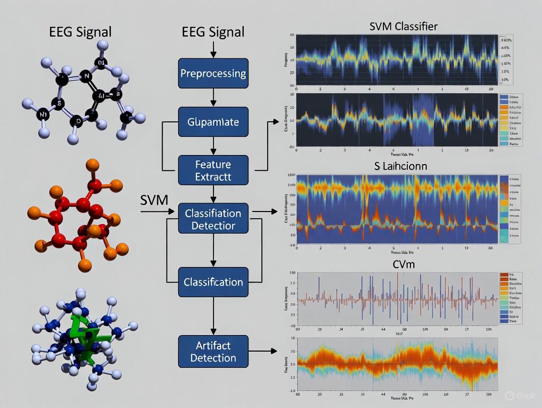
Workflow Visualization for SVM-Based Artifact Detection
The following diagram illustrates a proposed integrated workflow for SVM-based artifact detection and removal, incorporating elements from the experimental protocols.
The Scientist's Toolkit: Research Reagent Solutions
This table details essential computational tools, datasets, and algorithms that form the "research reagents" for developing EEG artifact detection systems.
Table 3: Essential Resources for EEG Artifact Research
| Resource Name | Type | Function/Benefit | Example Use Case |
|---|---|---|---|
| EEGdenoiseNet [1] | Benchmark Dataset | Provides clean EEG and recorded EOG/EMG for creating semi-synthetic data. | Training and benchmarking supervised models like SVM. |
| TUH EEG Artifact Corpus [5] | Clinical EEG Dataset | Large, real-world dataset with expert-annotated artifact labels. | Testing model generalizability to clinical data. |
| RELAX (EEGLAB Plugin) [7] | Software Pipeline | Implements targeted artifact reduction to minimize false positives in ERPs. | Post-detection cleaning to preserve neural signals. |
| Grey Wolf Optimizer (GWO) [6] | Metaheuristic Algorithm | Reduces feature dimensionality, lowering computational cost for SVM. | Optimizing feature selection from a large extracted set. |
| Goose Optimization Algorithm [6] | Metaheuristic Algorithm | Optimizes the parameters of a hybrid SVM-Fuzzy classifier. | Fine-tuning classifier hyperparameters for high accuracy. |
| Lightweight CNN [5] | Deep Learning Model | Acts as a feature extractor; provides discriminative inputs for SVM. | Transfer learning for feature extraction from EEG epochs. |
| Independent Component Analysis (ICA) [2] [7] | Blind Source Separation | Decomposes EEG into independent components for analysis. | Identifying artifact-laden components for removal. |
Support Vector Machines (SVMs) represent a cornerstone of supervised machine learning models with particular significance for electroencephalography (EEG) analysis, including the critical task of artifact detection. Developed at AT&T Bell Laboratories and based on statistical learning frameworks of VC theory proposed by Vapnik and Chervonenkis, SVMs are max-margin models designed for classification and regression analysis [8]. In the context of EEG research, where distinguishing neural signals from artifacts remains challenging, SVMs provide distinct advantages due to their resilience to noisy data and strong generalization performance with limited samples [9] [8].
The application of SVM-based frameworks in EEG artifact detection has gained substantial research interest, particularly as wearable EEG technologies introduce new challenges with artifacts exhibiting specific features due to dry electrodes, reduced scalp coverage, and subject mobility [10]. Artifacts—unwanted signals originating from non-neural sources—can significantly compromise EEG interpretation and lead to clinical misdiagnosis if not properly identified [2]. SVM's capacity to handle high-dimensional, nonlinear data makes it particularly suited for differentiating subtle artifact patterns from genuine brain activity in complex EEG recordings [9] [11].
Core Theoretical Principles
Linear Separation and Maximum Margin Classification
The fundamental principle underlying SVM is the concept of optimal linear separation in a high-dimensional feature space. Given a training dataset of n points of the form {(x₁, y₁), ..., (xₙ, yₙ)}, where xᵢ represents the feature vectors and yᵢ ∈ {-1, 1} denotes class labels, SVM constructs a hyperplane that separates the two classes with maximum margin [8]. For EEG artifact detection, these two classes typically represent "clean EEG" versus "artifact-contaminated EEG," though multi-class extensions exist for identifying specific artifact types.
The optimal separating hyperplane satisfies the condition yᵢ(wᵀxᵢ - b) ≥ 1 for all i, where w is the weight vector normal to the hyperplane and b is the bias term. The margin width between classes is given by 2/‖w‖, which SVM maximizes while ensuring correct classification [8]. This maximum margin principle enhances the model's generalization capability—a critical advantage for EEG applications where data non-stationarity is common.
Table 1: Key Mathematical Components of Linear SVM
| Component | Mathematical Expression | Role in EEG Artifact Detection |
|---|---|---|
| Hyperplane | wᵀx - b = 0 | Decision boundary for artifact vs. clean EEG |
| Margin Width | 2/‖w‖ | Buffer zone maximizing robustness to EEG variability |
| Constraint | yᵢ(wᵀxᵢ - b) ≥ 1 | Ensures correct classification of training examples |
| Optimization | min┬(w,b) ½‖w‖² | Finds optimal separation with minimal misclassification |
Soft Margin and Hinge Loss for Noisy EEG Data
In practical EEG applications, perfect linear separation is often impossible due to noise and overlapping class distributions. The soft-margin formulation addresses this through the introduction of slack variables (ξᵢ) and a regularization parameter (C) [8]. The optimization problem becomes:
min┬(w,b,ξ) ½‖w‖² + C(∑ᵢξᵢ) subject to yᵢ(wᵀxᵢ - b) ≥ 1 - ξᵢ and ξᵢ ≥ 0
The hinge loss function, defined as max(0, 1 - yᵢ(wᵀxᵢ - b)), quantifies the misclassification error [8]. The parameter C controls the trade-off between maximizing the margin and minimizing classification errors—a crucial consideration for EEG artifact detection where some artifacts may share characteristics with neural signals.
Kernel Methods for Nonlinear EEG Pattern Recognition
The kernel trick represents SVM's most powerful capability for handling nonlinear patterns in EEG data. By mapping input features to a higher-dimensional space without explicit transformation, SVMs can construct nonlinear decision boundaries [8]. For a kernel function K(xᵢ, xⱼ) = φ(xᵢ)ᵀφ(xⱼ), the dual optimization problem becomes:
max┬(α) ∑ᵢαᵢ - ½∑ᵢ∑ⱼαᵢαⱼyᵢyⱼK(xᵢ, xⱼ) subject to 0 ≤ αᵢ ≤ C and ∑ᵢαᵢyᵢ = 0
Table 2: Common Kernel Functions in EEG Artifact Detection
| Kernel Type | Mathematical Form | Advantages for EEG Analysis |
|---|---|---|
| Linear | K(xᵢ, xⱼ) = xᵢᵀxⱼ | Interpretable, works well with high-dimensional features |
| Polynomial | K(xᵢ, xⱼ) = (γxᵢᵀxⱼ + r)ᵈ | Captures complex feature interactions in multi-channel EEG |
| Radial Basis Function (RBF) | K(xᵢ, xⱼ) = exp(-γ‖xᵢ - xⱼ‖²) | Handles nonlinear patterns common in artifact morphology |
| Multiple Kernel Learning | K(xᵢ, xⱼ) = ∑ₘdₘKₘ(xᵢ, xⱼ) | Combines heterogeneous EEG features optimally [9] |
Multiple Kernel Learning (MKL) represents an advanced approach where the kernel is defined as a linear combination of base kernels (e.g., polynomial and RBF), with weights dₘ optimized during training [9]. This approach has demonstrated promising results in EEG classification, achieving accuracies up to 99.20% for 2-class mental task discrimination [9].
SVM Applications in EEG Analysis and Artifact Detection
Performance in EEG Classification Tasks
SVMs have demonstrated exceptional performance across diverse EEG classification tasks. In mental task classification, MKL-SVM has achieved average accuracies of 99.20%, 81.25%, 76.76%, and 75.25% for 2-class, 3-class, 4-class, and 5-class classifications respectively [9]. For epilepsy detection, hybrid SVM models combining kernel sparse representation have reached over 99% accuracy in binary classification tasks, with certain applications attaining 100% accuracy [11].
In comparative studies, SVMs generally outperform other classifiers like Linear Discriminant Analysis (LDA) and Neural Networks (NN) for EEG-based Brain-Computer Interfaces (BCIs), particularly for solving problems with high dimensionality, nonlinearity, and small datasets [9] [12]. This superior performance stems from SVM's structural risk minimization principle, which contrasts with the empirical risk minimization approach of neural networks [9].
Artifact Detection and Correction Protocols
The impact of artifact correction on SVM decoding performance has been systematically evaluated across multiple experimental paradigms. Research demonstrates that the combination of artifact correction and rejection does not significantly enhance decoding performance in most cases, though artifact correction remains essential to minimize artifact-related confounds that might artificially inflate decoding accuracy [13].
Independent Component Analysis (ICA) has emerged as a preferred method for ocular artifact correction prior to SVM classification, while artifact rejection effectively discards trials with large voltage deflections from other sources such as muscle artifacts [13]. This protocol balance is particularly important for maintaining sufficient trial counts for SVM training while minimizing artifact contamination.
Advanced SVM Architectures for EEG Analysis
Recent research has explored hybrid architectures integrating SVMs with other methodologies to enhance EEG analysis:
SVM-KSRC: A hybrid approach connecting SVM with Kernel Sparse Representation Classification using support vectors, demonstrating superior performance in epilepsy detection compared to either method used separately [11].
SVM-enhanced Attention Mechanisms: Integration of SVM's margin maximization objective directly into self-attention computation to improve interclass separability in motor imagery EEG classification [14].
Adaptive SVM (A-SVM): Online recursive updating of classifier parameters to address EEG non-stationarity, enabling the model to track changing feature distributions during prolonged recordings [12].
ORICA-CSP with A-SVM: Combination of Online Recursive Independent Component Analysis with Common Spatial Patterns and Adaptive SVM for robust feature extraction in motor imagery tasks [12].
Experimental Protocols and Methodologies
Standardized Protocol for EEG Artifact Detection Using SVM
Objective: To detect and classify artifacts in EEG signals using Support Vector Machines while preserving neural signals of interest.
Materials and Equipment:
- EEG recording system (wet or dry electrodes)
- Reference electrodes for EOG/EMG monitoring
- Preprocessing software (EEGLAB, FieldTrip, or custom tools)
- Computing environment with SVM implementation (Python scikit-learn, LIBSVM)
Procedure:
- Data Acquisition and Preprocessing
- Record EEG using standard montages (10-20 system or wearable configurations)
- Apply bandpass filtering (0.5-45 Hz) to remove extreme frequency artifacts
- Segment data into epochs relevant to experimental paradigm
- Implement average or reference electrode re-referencing
- Artifact Correction Phase
- Perform Independent Component Analysis (ICA) to separate neural and artifactual components
- Identify and remove components corresponding to ocular artifacts
- Apply correction to all channels while preserving neural activity [13]
- Feature Extraction
- Extract temporal features: variance, mean, amplitude, Hjorth parameters
- Calculate frequency-domain features: band power (delta, theta, alpha, beta, gamma)
- Compute complexity measures: entropy, fractal dimension, wavelet coefficients
- For multi-channel EEG: derive spatial features using CSP or Laplacian filters
- SVM Training and Validation
- Partition data into training (70%), validation (15%), and test (15%) sets
- Select appropriate kernel function based on data characteristics
- Optimize hyperparameters (C, γ) using grid search with cross-validation
- Train SVM model on artifact-labeled training data
- Evaluate performance on held-out test set using accuracy, sensitivity, specificity
- Implementation Considerations
- For wearable EEG with limited channels (<16), prioritize feature selection to avoid dimensionality issues [10]
- For real-time applications, implement adaptive SVM with periodic model updates [12]
- For multi-class artifact identification, employ one-vs-one or one-vs-rest strategies
Protocol for Multi-class Mental Task Classification Using MKL-SVM
Objective: To classify multiple cognitive states from EEG signals using Multiple Kernel Learning SVM [9].
Procedure:
- EEG Preprocessing
- Apply artifact correction using ICA
- Bandpass filter to 0.5-40 Hz range
- Segment data into task-specific epochs
- Multi-domain Feature Extraction
- Compute Wavelet Packet Entropy (WPE) for time-frequency analysis
- Calculate Granger causality for effective connectivity between channels
- Extract power spectral density across standard frequency bands
- Multiple Kernel Configuration
- Define base kernels: polynomial (degree 2-3) and RBF (varying γ)
- Initialize kernel weights uniformly: dₘ = 1/M for m = 1,...,M
- Implement gradient descent optimization to learn optimal kernel weights
- Model Training and Evaluation
- Employ K-fold cross-validation (typically K=10)
- Use SimpleMKL algorithm for efficient optimization [9]
- Evaluate using classification accuracy, F1-score, and confusion matrix analysis
The Scientist's Toolkit: Research Reagent Solutions
Table 3: Essential Resources for SVM-Based EEG Artifact Detection Research
| Resource Category | Specific Examples | Research Application |
|---|---|---|
| EEG Datasets | BCI Competition IV (Dataset 2a, 2b), University of Bonn Epilepsy Dataset, Physionet EEG Motor Movement/Imagery Dataset | Benchmarking SVM performance across different artifact types and EEG paradigms [11] [15] |
| Artifact Processing Tools | Independent Component Analysis (ICA), Automatic Subspace Reconstruction (ASR), Wavelet Transform Denoising | Preprocessing to isolate artifacts and enhance signal quality before SVM classification [13] [10] |
| Feature Extraction Algorithms | Common Spatial Patterns (CSP), Wavelet Packet Entropy (WPE), Granger Causality, Empirical Mode Decomposition (EMD) | Generating discriminative features for SVM classification of artifacts vs. neural signals [9] [12] [15] |
| SVM Implementations | LIBSVM, scikit-learn SVC, SimpleMKL, Adaptive SVM (A-SVM) | Core classification algorithms with varying kernel options and adaptation capabilities [9] [12] |
| Performance Metrics | Accuracy, Sensitivity, Specificity, F1-Score, Area Under ROC Curve (AUC) | Quantifying artifact detection performance and model comparison [10] [11] |
| Validation Methodologies | Leave-One-Subject-Out (LOSO) Cross-Validation, K-fold Cross-Validation, Hold-out Validation | Ensuring robust generalizability of SVM models across subjects and sessions [14] [15] |
Support Vector Machines provide a powerful framework for EEG artifact detection, offering robust performance through their maximum margin principle and kernel-based nonlinear mapping capabilities. From fundamental linear separation to advanced multiple kernel learning approaches, SVMs continue to evolve with hybrid architectures that address the unique challenges of EEG analysis. As wearable EEG technologies advance and artifact management grows more complex, SVM-based methodologies remain essential tools for researchers seeking to extract meaningful neural information from contaminated signals. The continued integration of SVMs with adaptive learning, deep learning architectures, and multimodal signal processing promises to further enhance their utility in both clinical and research applications.
Why SVM for EEG? Advantages in Handling Non-Stationary and High-Dimensional Neural Data
Electroencephalogram (EEG) signals represent one of the most complex biological datasets, characterized by inherent non-stationarity, high dimensionality, and low signal-to-noise ratio. These characteristics pose significant challenges for pattern recognition algorithms in brain-computer interfaces (BCIs), neurological disorder diagnosis, and cognitive state monitoring. Among various machine learning approaches, Support Vector Machines (SVM) have demonstrated consistent effectiveness across diverse EEG applications, from motor imagery classification to epileptic seizure detection and neurological disease diagnosis. The theoretical foundation of SVM, based on statistical learning theory and structural risk minimization, provides distinct advantages for EEG data analysis compared to other classification approaches [16] [17] [18].
Performance Comparison: SVM vs. Other Classification Methods
Table 1: Comparative Performance of SVM and Other Classifiers on EEG Tasks
| EEG Application | SVM Performance | Alternative Methods | Comparative Performance |
|---|---|---|---|
| Motor Imagery Classification | 91% accuracy [19] | Random Forest: 91% [19] | Equivalent top performance |
| Epileptic Seizure Detection | 99% accuracy [20] | Naïve Bayes: 96.47% [20] | SVM superior by ~2.5% |
| Epileptic Seizure Recognition | 99.42% accuracy (CNN-SVM-PCA) [20] | DNN alone: 96.91% [20] | Hybrid SVM superior by ~2.5% |
| Ictal EEG Detection | 97% sensitivity, 96.25% specificity [18] | EMD with other classifiers | State-of-the-art performance |
| Alzheimer's Detection | ~3% improvement with SVM classifier [21] | Deep learning models alone | Consistent performance enhancement |
| Artifact Correction | No significant improvement from artifact rejection [13] | Multiple artifact handling methods | Robust to artifact correction |
Table 2: SVM Performance Across EEG Datasets and Conditions
| Dataset | SVM Variant | Feature Extraction | Performance Metrics |
|---|---|---|---|
| BCI Competition III [16] | PSO-optimized SVM | Common Spatial Patterns | Significant improvement in classification accuracy |
| Bonn EEG Dataset [18] | Standard SVM | Empirical Mode Decomposition | 98% sensitivity, 99.4% specificity |
| Epileptic Seizure Recognition [20] | CNN-SVM-PCA | Deep Learning + PCA | 99.42% accuracy |
| BONN Dataset [20] | CNN-SVM-PCA | Deep Learning + PCA | 99.96% accuracy |
| Clinical EEG Data [17] | Universum SVM | Wavelet Transform | 99% classification accuracy |
Theoretical Advantages of SVM for EEG Analysis
Handling High-Dimensional Data
EEG data typically involves recordings from multiple channels (often 32-256) across time samples, creating feature spaces with extremely high dimensionality. SVM excels in such environments through kernel tricks that map data to higher-dimensional spaces where linear separation becomes feasible without explicitly computing the coordinates in that space [16] [17]. This capability allows SVM to handle the complex interactions between EEG channels and time points effectively.
Managing Limited Training Samples
Unlike deep learning approaches that typically require large datasets, SVM performs effectively with relatively small training samples, which is particularly valuable in EEG research where data collection is often constrained by subject availability, fatigue, and experimental practicality [16] [22]. The structural risk minimization principle implemented in SVM seeks to minimize the upper bound of generalization error rather than just training error, enhancing performance on limited datasets [17].
Robustness to Non-Stationarity
EEG signals are inherently non-stationary, with statistical properties that change over time due to brain state transitions, artifacts, and other factors. SVM's margin maximization provides inherent robustness to certain types of variability and noise, as small perturbations in the input space typically do not significantly affect the optimal hyperplane [14] [13].
Global Optimization Solution
The convex optimization formulation of SVM guarantees a global optimum, avoiding the local minima problems that plague neural network approaches. This reliability is particularly valuable in clinical and research applications where consistent performance is essential [17].
Experimental Protocols for EEG Classification with SVM
Standard Protocol for Motor Imagery EEG Classification
Protocol Details:
Data Acquisition and Preprocessing
- Collect EEG signals using standard international 10-20 electrode placement system
- Apply band-pass filtering between 0.5-40 Hz to remove high-frequency noise and DC drift
- Perform artifact removal using Independent Component Analysis (ICA) or regression methods
- Segment data into epochs time-locked to motor imagery cues
Feature Extraction using Common Spatial Patterns (CSP)
- Calculate spatial covariance matrices for different motor imagery classes
- Perform simultaneous diagonalization of covariance matrices
- Select spatial filters that maximize variance for one class while minimizing for another
- Extract features as log-variance of CSP-filtered signals [16]
SVM Model Training and Optimization
- Utilize RBF kernel for nonlinear classification boundaries
- Optimize kernel parameters (γ) and regularization (C) using grid search or PSO
- Implement cross-validation strategies appropriate for EEG (e.g., leave-one-subject-out)
- Train final model on optimized parameters
Advanced Protocol: SVM-Enhanced Deep Learning for EEG
Protocol Details:
Hybrid Architecture Integration
- Implement CNN layers for spatial feature extraction from multichannel EEG
- Utilize LSTM or BiLSTM networks for temporal dynamics modeling
- Integrate SVM principles directly into attention mechanisms to enhance class separability
- Replace traditional softmax output with SVM-based margin classification [14]
SVM-Enhanced Attention Mechanism
- Embed margin maximization objective directly into self-attention computation
- Transform standard attention to maximize separation between class centroids
- Apply regularization that enforces large margin between different motor imagery classes
- This approach has demonstrated consistent improvements in accuracy, F1-score, and sensitivity compared to conventional attention mechanisms [14]
Implementation Considerations
- Use differentiable quadratic programming solutions for SVM integration
- Implement custom loss functions combining cross-entropy and margin terms
- Balance contributions of deep learning and SVM components through weighted losses
Research Reagent Solutions: Essential Tools for EEG-SVM Research
Table 3: Key Computational Tools and Algorithms for EEG-SVM Research
| Research Tool | Function | Application Context |
|---|---|---|
| Common Spatial Patterns (CSP) | Spatial filter optimization | Motor imagery feature extraction [16] |
| Regularized CSP (RCSP) | Improved covariance estimation | Small sample size scenarios [16] |
| Empirical Mode Decomposition (EMD) | Non-stationary signal decomposition | Epileptic seizure detection [18] |
| Particle Swarm Optimization (PSO) | Hyperparameter optimization | SVM kernel and parameter selection [16] |
| Universum SVM | Incorporation of prior knowledge | Seizure classification with interictal data [17] |
| Wavelet Transform | Time-frequency analysis | Feature extraction for neurological disorders [17] |
| Independent Component Analysis (ICA) | Artifact removal and source separation | EEG preprocessing [13] [4] |
| Riemannian Geometry | Manifold-based classification | Advanced feature space transformation [19] |
Discussion: SVM in Modern EEG Research Context
While deep learning approaches have gained prominence in EEG analysis, SVM continues to offer distinct advantages, particularly in scenarios with limited training data, requirement for model interpretability, or computational constraints. The emergence of hybrid models that combine deep learning feature extraction with SVM classification demonstrates the ongoing relevance of SVM in advanced BCI and neurotechnology applications [14] [20].
Recent research has successfully integrated SVM with deep learning architectures, creating models that leverage the complementary strengths of both approaches. These hybrid systems typically use deep neural networks for automatic feature learning from raw or minimally processed EEG signals, while employing SVM in the final classification layer to provide robust decision boundaries with strong generalization capabilities [14] [20].
Furthermore, SVM's well-established theoretical foundation provides interpretability advantages over pure deep learning models, which often function as "black boxes." This interpretability is particularly valuable in clinical applications and scientific research where understanding the relationship between EEG features and classification outcomes is essential for validation and trust in the system [17] [18].
Support Vector Machines remain a powerful and relevant tool for EEG signal classification, offering proven performance across diverse applications from basic research to clinical diagnostics. Their theoretical foundations in statistical learning theory provide inherent advantages for handling the high-dimensional, non-stationary, and noisy nature of neural data. While pure SVM approaches deliver robust performance, particularly with appropriate feature engineering, the future trajectory points toward hybrid models that leverage deep learning for feature representation and SVM for robust classification. This synergistic approach combines the representational power of neural networks with the generalization guarantees of margin-based classifiers, pushing the boundaries of what's possible in EEG decoding and brain-computer interface technology.
The Critical Impact of Artifacts on Downstream Analysis in Drug Development Pipelines
In the high-stakes environment of drug development, the integrity of analytical data is paramount. Artifacts—systematic errors and non-biological noise—introduced during experimental procedures represent a critical, yet often undetected, threat to data reliability and subsequent decision-making. These artifacts can originate from various sources, including instrumental errors, environmental factors, and procedural inconsistencies, ultimately compromising the validity of downstream analyses and potentially derailing development pipelines. Traditional quality control (QC) methods, which primarily rely on control wells, have proven insufficient for detecting many spatial and systematic artifacts that specifically affect drug-treated samples [23].
This application note examines the profound impact of artifacts on drug development data, highlighting a novel QC metric—Normalized Residual Fit Error (NRFE)—that directly addresses this challenge. Furthermore, we explore the translational potential of advanced artifact detection methodologies, specifically Support Vector Machine (SVM)-based frameworks successfully applied in electroencephalography (EEG) signal processing, for enhancing reliability in pharmaceutical screening. We provide detailed protocols and resources to empower researchers to identify, quantify, and mitigate artifacts, thereby safeguarding data integrity from initial discovery through to regulatory submission.
The Hidden Problem: Undetected Artifacts in Drug Screening
Large-scale pharmacogenomic initiatives, such as the Cancer Cell Line Encyclopedia (CCLE) and Genomics of Drug Sensitivity in Cancer (GDSC), have significantly advanced our understanding of drug responses. However, concerns regarding inter-laboratory consistency and reproducibility persist, often traceable to undetected artifacts in high-throughput screening (HTS) data [23]. Conventional QC metrics like Z-prime factor (Z'), Strictly Standardized Mean Difference (SSMD), and signal-to-background ratio (S/B) focus exclusively on control wells. This fundamental limitation renders them blind to systematic errors—such as evaporation gradients, pipetting inaccuracies, or drug-specific precipitation—that manifest specifically in drug wells [23].
The normalized residual fit error (NRFE) metric was developed to overcome this blind spot. By analyzing deviations between observed and fitted dose-response values across all compound wells and applying a binomial scaling factor to account for response-dependent variance, NRFE directly evaluates data quality from the drug-treated wells themselves [23]. This control-independent approach is orthogonal to traditional methods, making it particularly effective at identifying spatial artifacts and systematic errors that conventional metrics miss.
Table 1: Comparison of Traditional and NRFE Quality Control Metrics
| Metric | Basis of Calculation | Primary Strength | Primary Weakness |
|---|---|---|---|
| Z'-factor | Variability and separation of positive/negative controls [23] | Simple, established industry standard for assay-wide technical issues [23] | Cannot detect artifacts in drug wells; blind to spatial patterns [23] |
| SSMD | Normalized difference between controls [23] | Robust metric for effect size between controls [23] | Fails to capture drug-specific or position-dependent errors [23] |
| S/B Ratio | Ratio of mean control signals [23] | Simple to calculate and interpret [23] | Ignores variability; weakest correlation with other QC metrics [23] |
| NRFE | Deviations between observed and fitted dose-response values in all compound wells [23] | Detects systematic spatial artifacts and drug-specific issues missed by control-based metrics [23] | Requires dose-response data; not a replacement for control-based metrics (complementary) [23] |
The consequences of undetected artifacts are severe. Analysis of the PRISM dataset demonstrated that plates with elevated NRFE values (>15) exhibited a three-fold lower reproducibility among technical replicates compared to high-quality plates (NRFE <10) [23]. Furthermore, integrating NRFE into the QC process for matched data from the GDSC project improved the cross-dataset correlation from 0.66 to 0.76, underscoring its power to enhance data consistency and reliability [23]. The following workflow diagram illustrates how systematic artifacts undermine data integrity and how NRFE detects them.
Figure 1: Data Integrity Workflow. This diagram contrasts the ideal experimental workflow with the reality of how undetected artifacts lead to flawed conclusions, and how integrating NRFE into the QC process safeguards downstream analysis and reproducibility.
Translational Insights: SVM-Based Artifact Detection from EEG Research
The challenge of separating meaningful signal from complex noise is not unique to drug development. The field of neuroscience, particularly EEG analysis, has made significant strides in developing sophisticated computational methods for artifact detection and correction. The translational application of these methods holds great promise for pharmaceutical analytics.
SVM and Hybrid Models in EEG
In EEG research, artifacts from ocular, cardiac, and muscular activity profoundly complicate the interpretation of neural signals [24]. Support Vector Machines (SVMs) are a well-established machine learning technique for classifying clean EEG signals from contaminated ones. Their ability to handle high-dimensional data makes them particularly suitable for this task [6]. Research has demonstrated that a hybrid SVM-Fuzzy system, optimized with nature-inspired algorithms, can achieve exceptional accuracy (98.1%) in identifying epileptic seizures from EEG data, showcasing the power of combining SVM with complementary machine learning approaches for robust signal classification [6].
Furthermore, a critical study evaluating artifact minimization for EEG decoding concluded that while artifact correction (e.g., using Independent Component Analysis) is essential to avoid artificially inflated decoding accuracy, its combination with artifact rejection did not significantly enhance the performance of SVM-based decoders in most cases [13]. This highlights the robustness of SVM classifiers and underscores the primary importance of artifact correction prior to analysis.
The Power of Transfer Learning
A key advancement in artifact detection is the use of transfer learning. A seminal study demonstrated that an SVM artifact detection model trained on contact ECG data could be effectively optimized for a different signal modality—capacitively coupled ECG (ccECG)—using transfer learning [25]. This approach improved the classifier's accuracy on the new modality by 5-8%, requiring only a limited amount of newly labelled data (as few as 20 segments) for adaptation [25]. This methodology directly addresses a major bottleneck in drug development: the costly and time-consuming need to manually label large, modality-specific datasets for each new assay or instrument platform.
Integrated Application Protocol: Combining NRFE and SVM for Enhanced QC
This protocol outlines a hybrid quality control strategy that integrates the NRFE metric with an SVM classifier, leveraging the strengths of both approaches to maximize the detection of artifacts in drug screening data.
Protocol: NRFE-Guided SVM for Artifact Detection in HTS
Aim: To implement a two-tiered quality control pipeline for high-throughput drug screening that identifies both systematic spatial artifacts (via NRFE) and complex, non-linear signal contaminants (via SVM).
Materials and Reagents
- Drug Plates: 384-well or 96-well microplates containing test compounds and controls.
- Cell Lines: Relevant cancer or disease-specific cell lines.
- Viability/Range Readout Kit: e.g., CellTiter-Glo Luminescent Cell Viability Assay.
- Automated Liquid Handling System.
- Plate Reader: Compatible with the chosen readout kit.
- Software: R package
plateQCfor NRFE calculation [23]; Python with scikit-learn for SVM modeling; specialized tool for dose-response curve fitting (e.g.,drcin R).
Procedure
- Step 1: Experimental Setup & Data Acquisition
- Seed cells into microplates according to standard protocols for your cell line and assay.
- Dispense compounds across the plate using the liquid handling system, ensuring a logical dose-response pattern (e.g., serial dilutions across a row or column).
- Incubate for the designated time and develop the assay according to the readout kit's instructions.
- Acquire raw data (e.g., luminescence, fluorescence) from the plate reader.
Step 2: Calculate Traditional and NRFE QC Metrics
- Calculate traditional QC metrics (Z'-factor, SSMD) from the positive and negative control wells [23].
- Fit dose-response curves to the raw data for each compound-cell line combination.
- Using the
plateQCR package, compute the NRFE value for each plate using the fitted and observed values [23]. - QC Checkpoint 1: Apply tiered NRFE thresholds. Flag plates with NRFE > 15 for exclusion or expert review. Plates with NRFE between 10-15 require additional scrutiny, while those with NRFE < 10 are considered acceptable [23].
Step 3: Prepare Data for SVM Classification
- From the raw well-level data, extract a set of signal quality features. These can include:
- Label a subset of data segments (e.g., wells or plate sectors) as "clean" or "contaminated" based on the NRFE analysis and visual inspection to create a training set.
Step 4: Train and Apply SVM Classifier
- Train an SVM model with a radial basis function (RBF) kernel on the labeled feature data from a source domain (e.g., a previously validated HTS dataset or a different modality).
- Optional Transfer Learning: If the model performance on a new target domain (e.g., a novel assay format) is suboptimal, apply transfer learning. Use a small set of labeled data from the new domain to adapt the pre-trained SVM model, fine-tuning its decision boundary [25].
- Use the trained (or adapted) SVM model to classify all wells or segments in the dataset.
Step 5: Integrated Decision Making
- Combine the results from the NRFE and SVM analyses. A plate should be considered for rejection or re-testing if it is flagged by either method.
- This integrated approach ensures the detection of both large-scale systematic artifacts (NRFE's strength) and localized or complex signal contaminants (SVM's strength).
The following workflow provides a visual summary of this integrated protocol.
Figure 2: Integrated NRFE-SVM QC Protocol. This workflow diagram outlines the parallel paths of NRFE-based plate assessment and SVM-based signal classification, which converge for a final, robust data quality assessment.
The Scientist's Toolkit: Key Research Reagents & Solutions
Table 2: Essential Materials for Implementing Advanced Artifact Detection
| Item | Function/Description | Example/Supplier |
|---|---|---|
| plateQC R Package | Open-source software for calculating the NRFE metric and performing control-independent quality assessment of drug screening plates [23]. | Available at: https://github.com/IanevskiAleksandr/plateQC [23] |
| SVM Library | A robust programming library for creating and training Support Vector Machine classifiers for signal quality assessment. | Python's scikit-learn (sklearn.svm.SVC) |
| Dose-Response Curve Fitting Tool | Software for modeling the relationship between compound concentration and effect, which is a prerequisite for NRFE calculation. | R package drc |
| High-Quality Control Compounds | Well-characterized agonists/antagonists for establishing robust positive and negative controls, ensuring traditional QC metrics (Z', SSMD) are valid. | Supplier-specific (e.g., Tocris, Sigma-Aldrich) |
| Standardized Cell Viability Assay | A homogeneous, luminescent assay for quantifying viable cells, providing a reproducible readout for HTS. | CellTiter-Glo Luminescent Assay |
Artifacts pose a silent but critical threat to the integrity of the drug development pipeline. While traditional QC methods provide a foundational check, they are inadequate for detecting the full spectrum of systematic errors. The integration of novel, control-independent metrics like NRFE and the strategic adoption of robust machine learning classifiers, such as SVMs, offer a powerful, multi-layered defense. By learning from adjacent fields like EEG signal processing and implementing the detailed protocols and tools outlined in this document, drug development professionals can significantly enhance data reliability, improve reproducibility between studies, and de-risk the entire pipeline from discovery to clinical application.
From Theory to Practice: Implementing SVM Pipelines for EEG Artifact Detection
The efficacy of Support Vector Machine (SVM) models in electroencephalography (EEG) artifact detection hinges critically on appropriate data preprocessing. EEG signals are inherently non-stationary and contaminated by various biological and environmental artifacts, including ocular movements, muscle activity, and power line interference [4]. Without meticulous preprocessing, these artifacts can masquerade as genuine neural patterns, leading to misleading SVM classification results. Proper preprocessing transforms raw, artifact-laden EEG signals into a feature space where the SVM can construct an optimal hyperplane to distinguish genuine neural activity from artifacts, thereby enhancing the model's generalization capability and physiological interpretability [26]. This document outlines standardized protocols for filtering, segmentation, and feature extraction strategies specifically optimized for SVM-based artifact detection in EEG research.
Data Preprocessing Pipeline for SVM
Filtering and Artifact Removal
Table 1: Filtering Techniques for EEG Artifact Management
| Technique | Primary Function | Parameters | Impact on SVM Performance |
|---|---|---|---|
| Bandpass Filter | Removes non-physiological frequencies | 0.5-45 Hz for neural signals; 4-13 Hz for muscular artifacts [10] | Reduces high-frequency noise that can dominate SVM feature space |
| Wavelet Transform | Multi-resolution analysis for non-stationary artifacts | Mother wavelet: Daubechies; Threshold: Stein's Unbiased Risk Estimate [27] | Preserves transient neural features while removing artifacts |
| Independent Component Analysis (ICA) | Separates neural and artifactual sources | InfoMax or Extended-Infomax algorithm [10] | Isforms artifact-related components for rejection |
| Automatic Subspace Reconstruction (ASR) | Corrects large-amplitude artifacts | Cutoff: 20-30 standard deviations [10] | Handles movement and transient artifacts in continuous EEG |
| Deep Learning (AnEEG) | Artifact removal via LSTM-based GAN | Generator: 2-layer LSTM; Discriminator: 4-layer 1D-CNN [4] | Generates artifact-free signals while preserving neural dynamics |
Temporal Segmentation Strategies
Table 2: EEG Segmentation Methods for SVM Analysis
| Method | Principle | Parameters | SVM Compatibility |
|---|---|---|---|
| Fixed-Length Segmentation | Divides EEG into equal epochs | 0.5-2 second windows; 50% overlap optional [28] | Simple implementation; Consistent feature vector dimensions |
| Adaptive Segmentation (CTXSEG) | Creates variable-length segments based on statistical differences | Change point detection; Stationarity-based boundaries [28] | May require feature normalization for fixed SVM input dimensions |
| Functional Connectivity Segmentation | Segments based on network structure stability | Connectivity metric: PLV/PC; Graph distance threshold [29] | Captures cognitive state changes relevant to artifact detection |
| Event-Locked Segmentation | Epochs aligned to external events | Pre/post-event intervals; Baseline correction | Controls for event-related potentials in artifact detection |
Feature Extraction for SVM Optimization
Feature extraction transforms preprocessed EEG signals into discriminative representations that enable SVMs to effectively separate artifactual from neural components.
Time-Domain Features: Include statistical measures (variance, skewness, kurtosis) and amplitude-based features that capture artifact characteristics such as abrupt voltage deflections from ocular movements [27].
Frequency-Domain Features: Power spectral density estimates across standard bands (delta, theta, alpha, beta, gamma) help identify artifacts with distinct spectral signatures, such as muscle contamination in high-frequency bands [27].
Time-Frequency Features: Wavelet coefficients provide joint temporal and spectral information crucial for detecting transient artifacts like eye blinks that have both temporal localization and frequency content [27].
Nonlinear Features: Entropy measures (Fuzzy Entropy, Hierarchical Fuzzy Entropy) and fractal dimensions quantify signal complexity, with artifacts often exhibiting different regularity patterns compared to neural signals [30].
Spatial Features: For multi-channel EEG, common spatial patterns (CSP) and functional connectivity metrics capture topographic distributions that differentiate localized artifacts from distributed neural activity [12].
Experimental Protocols
Protocol 1: Comprehensive Artifact Processing Pipeline
Objective: Implement a complete artifact detection and correction pipeline for SVM-based EEG analysis.
Materials: Raw EEG data (minimum 16 channels), MATLAB/Python with EEGLAB, SVM library (scikit-learn), high-performance computing resources.
Procedure:
- Data Import: Load raw EEG data in standard format (e.g., .edf, .set).
- Bandpass Filtering: Apply 0.5-45 Hz zero-phase bandpass filter.
- Bad Channel Identification: Detect channels with excessive noise (>5 SD from mean).
- ICA Decomposition: Perform ICA using InfoMax algorithm.
- Artifact Component Classification: Use ICLabel to identify artifact-related components.
- Component Removal: Subtract ocular and muscular artifact components.
- Segmentation: Apply fixed-length segmentation (1-second epochs, no overlap).
- Feature Extraction: Compute time-domain, frequency-domain, and nonlinear features.
- SVM Training: Train linear SVM with 5-fold cross-validation.
- Performance Validation: Assess accuracy, sensitivity, specificity on held-out test set.
Troubleshooting: If SVM performance is suboptimal, consider alternative segmentation strategies or feature sets. For computational efficiency with large datasets, consider ASR as an alternative to ICA [10].
Protocol 2: Adaptive Segmentation for Non-Stationary EEG
Objective: Implement and validate adaptive segmentation to improve artifact detection in continuous EEG.
Materials: Continuous EEG recording, MATLAB/Python with signal processing toolbox, custom segmentation algorithms.
Procedure:
- Preprocessing: Apply basic bandpass filter (0.5-45 Hz).
- Functional Connectivity Calculation: Compute phase locking value (PLV) between all channel pairs using sliding window (0.5s duration).
- Graph Distance Computation: Calculate network structure differences between consecutive windows using node centrality measures [29].
- Change Point Detection: Identify segmentation boundaries where graph distance exceeds 2 standard deviations from mean.
- Segment Validation: Ensure minimum segment duration of 0.5s for meaningful analysis.
- Feature Extraction: Compute feature vectors for each variable-length segment.
- Feature Normalization: Apply standardization to accommodate variable segment lengths for SVM.
- SVM Classification: Train and test SVM on adaptive segments compared to fixed segments.
Validation: Compare classification performance between fixed and adaptive segmentation using ROC analysis.
Visualization of Workflows
EEG Processing Pipeline for SVM
Artifact Detection Decision Protocol
Table 3: Critical Resources for EEG Artifact Detection Research
| Resource | Specification | Research Application |
|---|---|---|
| EEG Acquisition System | 64-channel wet electrode system with impedance <10 kΩ | Gold-standard reference data collection [10] |
| Wearable EEG Headset | Dry electrode system with motion sensors | Ecological artifact data collection [10] |
| EEGLAB Toolkit | MATLAB-based environment with ICA implementation | Standardized preprocessing and component analysis [13] |
| BCI Competition IV Dataset 2a | 9-subject, 4-class motor imagery data | Benchmark for artifact detection algorithms [12] |
| PhysioNet Motor Imagery Dataset | 64-channel EEG from 109 subjects | Large-scale validation of SVM approaches [4] |
| Custom SVM Implementation | Scikit-learn with linear and RBF kernels | Flexible model development and testing [26] |
Effective preprocessing pipelines are fundamental to robust SVM-based EEG artifact detection. The integration of advanced filtering techniques, adaptive segmentation approaches, and multidimensional feature extraction creates an optimized pathway for distinguishing artifacts from neural signals. Current evidence suggests that while artifact correction is essential to minimize confounds, the combination of correction and rejection does not necessarily enhance SVM decoding performance in all paradigms [13]. Future research directions should focus on real-time adaptive processing, deep learning integration for artifact removal [4], and standardized benchmarking across diverse EEG acquisition systems. The protocols outlined herein provide a foundation for reproducible, effective artifact detection in SVM-based EEG research.
Electroencephalography (EEG) is a vital tool in neuroscience and clinical diagnostics, but its signal quality is often compromised by artifacts—unwanted noise originating from both physiological and non-biological sources. Effective artifact detection is a critical preprocessing step, and Support Vector Machines (SVMs) have proven to be powerful classifiers for this task. The performance of an SVM model is heavily dependent on the features it receives; well-engineered features that capture the distinct characteristics of artifacts in the temporal, spectral, and spatial domains are paramount for high-accuracy detection. These features enable the SVM to construct optimal hyperplanes for separating artifact-contaminated EEG segments from clean brain activity. This document provides detailed application notes and protocols for feature engineering, framed within the context of a broader thesis on SVM-based artifact detection in EEG research.
Feature Engineering Domains and Quantitative Comparison
The following sections delineate feature extraction methodologies across three fundamental domains. The subsequent table provides a comparative summary of their performance and characteristics.
Table 1: Comparative Analysis of Feature Domains for SVM-Based Artifact Detection
| Domain | Example Features | Best for Artifact Type | Key Advantage | Reported Performance (Accuracy) |
|---|---|---|---|---|
| Temporal | Statistical Moments (Variance, Skewness, Kurtosis), Amplitude Threshold | Eye-blink, High-amplitude Glitches | Computational simplicity, real-time applicability | >90% for eye-blink (with topography) [31] |
| Spectral | Power Spectral Density (PSD), Band Power (Delta, Theta, Alpha, Beta, Gamma), Spectral Entropy | Muscle, Electrode Pop, Powerline Noise | Directly captures oscillatory nature of EEG and artifacts | Varies by artifact; PSD is a foundational feature [32] [27] |
| Spatial | Scalp Topography, Phase Locking Value (PLV), Functional Connectivity Maps | Eye-blink, Muscle, Channel-specific Noise | Exploits multi-channel information and brain network dynamics | 97.61% (for emotion detection, indicative of high utility) [33] |
| Time-Frequency | Wavelet Coefficients, Marginal Hilbert Spectrum (MHS) | Muscle, Motion, Complex Transients | Resolves non-stationary signals; high joint time-frequency resolution | Effective for muscular and motion artifacts [34] [33] |
Temporal Domain Features
Temporal domain features are computed directly from the EEG signal amplitude over time. They are computationally efficient and effective for detecting artifacts with distinct amplitude or statistical properties.
- Statistical Moments: These are fundamental descriptors of the signal's amplitude distribution.
- Variance/Standard Deviation: Measures signal power. Artifacts like eye-blinks or muscle bursts often cause large deviations from the mean, resulting in high variance.
- Skewness: Quantizes the asymmetry of the amplitude distribution. A symmetric brain signal typically has skewness near zero, while artifacts can introduce asymmetry.
- Kurtosis: Reflects the "tailedness" of the distribution. Signals with sharp, transient artifacts (e.g., spikes) often exhibit high kurtosis.
- Amplitude-based Features: Simple thresholds on the absolute amplitude or the peak-to-peak amplitude in an epoch can flag high-amplitude artifacts like electrode pops or large eye movements.
Spectral and Time-Frequency Domain Features
Spectral features characterize the frequency content of the EEG signal, which is crucial since both neural activity and artifacts occupy distinct frequency bands.
- Power Spectral Density (PSD): Estimates the power distribution across frequencies. It can be computed using methods like the Fast Fourier Transform (FFT) or Welch's method [27]. Muscle artifacts, for instance, manifest as a diffuse increase in high-frequency (Beta/Gamma) power.
- Band Power: The absolute or relative power within standard EEG bands (Delta: 0.5-4 Hz, Theta: 4-8 Hz, Alpha: 8-13 Hz, Beta: 13-30 Hz, Gamma: >30 Hz) is a highly informative feature [33] [32].
- Spectral Entropy: Measures the predictability or regularity of the power spectrum, with artifacts often introducing more disorder.
For non-stationary signals where frequency content changes over time, time-frequency analysis is superior.
- Wavelet Transform (WT): Decomposes the signal into different frequency components while retaining temporal information. Features can be extracted from the coefficients of specific scales corresponding to artifact-prone frequencies [34] [27]. Discrete Wavelet Transform (DWT) is widely used for its computational efficiency.
- Marginal Hilbert Spectrum (MHS): A component of the Hilbert-Huang Transform, MHS provides a time-frequency-energy representation that is highly effective for analyzing non-linear and non-stationary signals like EEG, showing promise for artifact detection [33].
Spatial Domain Features
Spatial features leverage information from multiple EEG electrodes to capture the topographic distribution of brain activity and artifacts.
- Scalp Topography: This feature captures the voltage map across the scalp at a given time point. Artifacts have characteristic topographic patterns; for example, eye-blink artifacts manifest as a strong, smooth frontal field that reverses polarity, a pattern easily distinguished from most cortical potentials. Research has identified scalp topography as the most potent single feature for detecting eye-blink artifacts [31].
- Functional Connectivity: These features quantify the statistical interdependence between signals from different electrode pairs, capturing the network dynamics of the brain.
- Phase Locking Value (PLV): A non-linear measure that assesses the consistency of phase differences between two signals over trials or time. It is used to construct functional connectivity maps that can distinguish artifact-related from brain-related activity [33].
- Other Measures: Correlation, coherence, and mutual information are also used to define connectivity and identify abnormal spatial patterns caused by artifacts.
Experimental Protocols for Feature Extraction
Protocol 1: Extraction of Spectral Features using Welch's PSD
Objective: To compute Power Spectral Density (PSD) and band power features from multi-channel EEG data for SVM training.
Materials:
- Cleaned, continuous or epoched EEG data.
- Computing environment (e.g., Python with MNE, SciPy, and Scikit-learn libraries).
Procedure:
- Data Segmentation: Divide the continuous EEG signal into non-overlapping or overlapping epochs (e.g., 2-second segments).
- Detrending: Remove linear trends from each epoch to prevent low-frequency drift from distorting the PSD estimate.
- Tapering: Apply a window function (e.g., Hanning window) to each epoch to reduce spectral leakage.
- FFT Computation: For each channel and epoch, compute the FFT.
- PSD Estimation: Calculate the squared magnitude of the FFT and normalize by the sampling frequency and window power to obtain the periodogram.
- Averaging: Average the periodograms across epochs (Welch's method) or across overlapping segments within a long epoch to reduce variance.
- Band Power Extraction: Integrate the PSD within the standard frequency bands (Delta, Theta, Alpha, Beta, Gamma) for each channel. These integrated values form the feature vector for each EEG segment.
SVM Integration: The band power values from all channels can be concatenated into a single feature vector for each data segment, which is then labeled (e.g., "clean" or "artifact") and used to train the SVM classifier [27].
Protocol 2: Extraction of Spatial Features using Functional Connectivity
Objective: To compute Phase Locking Value (PLV) between EEG channels and construct spatial feature vectors for artifact detection.
Materials:
- Preprocessed, band-pass filtered EEG data.
- Signal processing toolbox (e.g., MATLAB, Python with NumPy and MNE).
Procedure:
- Band Selection: Choose a frequency band of interest (e.g., Theta for eye-blinks, Gamma for muscle artifacts).
- Hilbert Transform: Apply the Hilbert transform to the band-pass filtered signal from each channel to extract the instantaneous phase, (\phi(t)), for each sample point.
- PLV Calculation: For each pair of channels (i) and (j), compute the PLV over a time window of length (T) as: (PLV{ij} = \left| \frac{1}{T} \sum{t=1}^{T} e^{i(\phii(t) - \phij(t))} \right|) where (i) is the imaginary unit. The result is a value between 0 (no phase synchronization) and 1 (perfect phase synchronization).
- Feature Vector Construction: The PLV values for all unique channel pairs are arranged into a symmetric connectivity matrix. The upper or lower triangle of this matrix (excluding the diagonal) can be unfolded into a feature vector that represents the spatial connectivity pattern for that time window [33].
SVM Integration: This PLV-based feature vector is labeled and used as input for the SVM. The classifier learns to distinguish the connectivity patterns associated with artifacts (e.g., highly synchronized frontal channels during an eye-blink) from those of clean, task-related brain activity.
Workflow Visualization: From Raw EEG to SVM Classification
The following diagram illustrates the integrated workflow for feature engineering and SVM-based artifact detection.
The Scientist's Toolkit: Research Reagents and Solutions
Table 2: Essential Materials and Tools for EEG Artifact Detection Research
| Item | Function in Research | Example/Note |
|---|---|---|
| High-Density EEG System | Acquires neural data with high spatial resolution. | 64+ channels; systems with active electrodes reduce environmental noise. |
| Dry-Electrode Wearable EEG | Enables data collection in ecological, real-world settings. | Prone to specific motion artifacts; requires tailored feature extraction [34]. |
| Independent Component Analysis (ICA) | Blind source separation to isolate artifact components. | Used as a preprocessing step to generate inputs for spatial feature extraction [35]. |
| Wavelet Toolbox | Provides algorithms for time-frequency decomposition. | MATLAB Wavelet Toolbox or Python PyWavelets for DWT/CWT analysis [27]. |
| Public EEG Datasets | Benchmarks and validates feature extraction methods. | DEAP, SEED, or artifact-annotated datasets are crucial for training SVMs [33] [36]. |
| SVM Libraries | Provides optimized implementations of the classifier. | libsvm, Scikit-learn (Python) with RBF kernel typically performs well. |
Electroencephalography (EEG) serves as a critical tool in clinical and neuroscientific research for non-invasively monitoring brain activity. However, EEG signals are notoriously susceptible to various artifacts—unwanted noise originating from ocular (EOG), muscular (EMG), cardiac (ECG), and environmental sources. These artifacts can obscure genuine neural activity and severely compromise the validity of subsequent analysis. Within the broader context of a thesis on Support Vector Machine (SVM) artifact detection in EEG research, this document outlines detailed application notes and protocols for designing, evaluating, and deploying a robust SVM-based pipeline for the identification and management of artifacts in EEG data. The structured workflow presented herein, from rigorous model training and cross-validation to final deployment, is designed to equip researchers, scientists, and drug development professionals with a reliable methodology to ensure the integrity of EEG-derived biomarkers in clinical trials and neurological studies.
SVM Workflow for EEG Artifact Detection
The following diagram illustrates the comprehensive workflow for an SVM-based system designed to detect artifacts in EEG data, integrating data handling, model development, and deployment phases.
SVM Workflow for EEG Artifact Detection
This workflow outlines the key stages for developing an SVM model to identify artifacts in EEG signals. The process begins with Raw EEG Data Acquisition, which is often contaminated with noise from various sources [37] [10]. The data then undergoes Signal Preprocessing, which may include bandpass filtering and specialized artifact removal techniques like Ensemble Empirical Mode Decomposition with Fast Independent Component Analysis (EEMD-FastICA) to effectively filter out EOG artifacts and other noise [37].
Subsequently, Feature Extraction is performed to capture discriminative characteristics from the preprocessed signals. For artifact detection, this often involves generating a comprehensive feature vector by integrating time-frequency features (e.g., using Wavelet Packet Transform - WPT) and nonlinear features (e.g., using Sample Entropy - SampEn) [37]. To enhance model efficiency and performance, Feature Selection techniques, such as Gray Wolf Optimization (GWO), can be employed to reduce dimensionality and select the most relevant features [6].
The core of the workflow is SVM Model Training, where a kernel function is selected, and hyperparameters are tuned. The model then undergoes rigorous Model Cross-Validation (e.g., k-Fold or Leave-One-Subject-Out - LOSO) to ensure performance generalizability and avoid overfitting [38] [39]. This is followed by comprehensive Model Evaluation using a suite of metrics like accuracy, precision, recall, F1-score, and AUC-ROC [40].
Finally, the validated model proceeds to Model Deployment, where it can be implemented for real-time artifact detection in wearable EEG systems [10] or for batch processing of recorded data, ultimately outputting Clean EEG Data or a detailed Artifact Report.
Experimental Protocols & Methodologies
Detailed Protocol: EEMD-FastICA for Ocular Artifact Removal
Objective: To remove ocular (EOG) artifacts from raw EEG signals, resulting in cleaner neural data [37].
- Step 1: Signal Decomposition. Apply Ensemble Empirical Mode Decomposition (EEMD) to the raw multi-channel EEG signal. EEMD adds white noise to the signal multiple times and performs Empirical Mode Decomposition (EMD) on each noisy version, then averages the results to obtain a set of stable Intrinsic Mode Functions (IMFs). This mitigates mode mixing and provides a more robust decomposition than standard EMD [37].
- Step 2: Source Separation. Use Fast Independent Component Analysis (FastICA) on the obtained IMFs. FastICA is a blind source separation algorithm that maximizes the non-Gaussianity of the components to isolate statistically independent sources, effectively separating neural activity from artifact components [37].
- Step 3: Artifact Identification & Reconstruction. Identify components corresponding to EOG artifacts based on their topographic maps and temporal characteristics. These components are then removed, and the remaining IMFs are reconstructed to produce a clean EEG signal with minimal EOG contamination [37].
Detailed Protocol: WPT-SampEn Feature Extraction for Fatigue Detection
Objective: To extract a robust set of features from preprocessed EEG signals for classifying driver fatigue states using an SVM [37].
- Step 1: Time-Frequency Decomposition. Perform Wavelet Packet Transform (WPT) on the artifact-reduced EEG signals. WPT provides a more detailed time-frequency representation than standard wavelet transform by decomposing both the approximation and detail coefficients, allowing for finer resolution across all frequency bands of interest (e.g., delta, theta, alpha, beta, gamma) [37].
- Step 2: Nonlinear Feature Calculation. Compute the Sample Entropy (SampEn) from the reconstructed EEG signals. SampEn is a measure of signal complexity and regularity. A decrease in SampEn is often associated with increased mental fatigue, providing a crucial nonlinear feature for the classifier [37].
- Step 3: Feature Vector Construction. Integrate the statistical features from WPT (e.g., energy, variance of coefficients) and the SampEn values into a comprehensive feature vector. This multi-feature fusion approach provides the SVM classifier with both time-frequency and nonlinear dynamic information, significantly improving detection accuracy for fatigue states [37].
Protocol: k-Fold Cross-Validation for Model Evaluation
Objective: To obtain a reliable and unbiased estimate of the SVM model's performance on unseen data [41] [39] [42].
- Step 1: Data Partitioning. Randomly shuffle the entire dataset and split it into 'k' equal-sized folds (a common choice is k=5 or k=10). For stratified k-fold, ensure each fold maintains the same proportion of class labels (e.g., artifact vs. clean) as the complete dataset, which is crucial for imbalanced data [41].
- Step 2: Iterative Training and Validation. For each unique fold 'i' (where i=1 to k):
- Use fold 'i' as the validation set.
- Use the remaining k-1 folds as the training set.
- Train the SVM model on the training set.
- Validate the trained model on the validation set and record the chosen performance metric(s) (e.g., accuracy, F1-score) [39].
- Step 3: Performance Averaging. Calculate the final performance estimate by averaging the results from the 'k' iterations. The standard deviation of these results indicates the model's stability across different data subsets [42].
Performance Metrics & Quantitative Data
Core Model Evaluation Metrics
Table 1: Key classification metrics for evaluating SVM performance in EEG artifact detection.
| Metric | Formula | Interpretation & Use-Case |
|---|---|---|
| Accuracy | (TP+TN)/(TP+TN+FP+FN) | Overall correctness. Best used on balanced datasets [40]. |
| Precision | TP/(TP+FP) | Measures the purity of positive predictions. Crucial when the cost of False Positives (FP) is high (e.g., mistakenly labeling clean EEG as artifact) [40] [42]. |
| Recall (Sensitivity) | TP/(TP+FN) | Measures the completeness of positive predictions. Crucial when the cost of False Negatives (FN) is high (e.g., failing to detect a true artifact) [40] [42]. |
| F1-Score | 2(PrecisionRecall)/(Precision+Recall) | The harmonic mean of Precision and Recall. Provides a single, balanced metric, especially useful for imbalanced datasets [40] [42]. |
| Specificity | TN/(TN+FP) | Measures the ability to identify negative cases correctly (true negative rate) [40]. |
| AUC-ROC | Area Under the ROC Curve | Measures the model's overall ability to discriminate between classes, independent of the classification threshold [40]. |
Reported Performance in EEG Studies
Table 2: Reported performance of SVM and hybrid models in recent EEG analysis studies.
| Study / Application | Methodology | Key Performance Outcome |
|---|---|---|
| Epileptic Seizure Detection [6] | Hybrid SVM-Fuzzy classifier with GWO feature selection | 98.1% Accuracy, 97.8% Sensitivity, 98.4% Specificity |
| Explainable Epilepsy Detection [38] | Feature engineering with kNN classifier (for context) | 99.61% Accuracy (10-fold CV), 79.92% Accuracy (LOSO CV) |
| Driver Fatigue Detection [37] | SVM with WPT and Sample Entropy features | Significant improvement in recognition accuracy compared to single-feature methods |
| Motor Imagery EEG Classification [14] | SVM-enhanced attention mechanism in a deep learning model | Consistent improvements in accuracy, F1-score, and sensitivity |
The Scientist's Toolkit: Research Reagent Solutions
Table 3: Essential computational tools and packages for implementing the SVM workflow.
| Tool / Solution | Function / Purpose | Example / Note |
|---|---|---|
| Signal Preprocessing Toolbox | Filtering, artifact removal, and basic time-frequency analysis. | EEGLAB, MNE-Python, FieldTrip (MATLAB) |
| Feature Extraction Library | Calculating complex, nonlinear, and entropy-based features. | PyEntropy (Python), Nonlinear Measures Toolbox |
| Machine Learning Framework | Implementing SVM, cross-validation, and hyperparameter tuning. | Scikit-learn (Python): provides SVC, cross_val_score, GridSearchCV [39] |
| Optimization Algorithm | For feature selection and hyperparameter optimization. | Gray Wolf Optimization (GWO), Goose Optimization Algorithm (GOA) [6] |
| Deep Learning Framework (Hybrid Models) | Building complex hybrid models (e.g., SVM-enhanced attention). | PyTorch, TensorFlow/Keras [14] |
| Visualization & Analysis Package | Generating plots, confusion matrices, and AUC-ROC curves. | Matplotlib, Seaborn (Python) |
Electroencephalography (EEG) is a fundamental tool for measuring brain activity, prized for its non-invasiveness, high temporal resolution, and cost-effectiveness [43] [44]. However, a significant challenge in EEG analysis is the susceptibility of the signals to diverse artifacts—recorded signals that do not originate from neural activity [2]. These artifacts, which can be physiological (e.g., from eye movements or muscle activity) or non-physiological (e.g., from electrical interference or electrode issues), obscure underlying brain activity and can severely compromise data interpretation [10] [2]. In clinical and research settings, this can lead to misdiagnosis or flawed scientific conclusions. The expansion of EEG into new domains like wearable devices and Brain-Computer Interfaces (BCIs) amplifies these challenges due to increased noise from motion and dry electrodes [10].
Support Vector Machines (SVMs) have emerged as a powerful tool to address this problem. As a supervised machine learning algorithm, SVM is adept at handling high-dimensional data and finding optimal boundaries between classes, making it particularly suitable for distinguishing clean EEG signals from various artifact types [6]. This application note details the use of SVM-based frameworks for artifact detection and removal across three critical scenarios: clinical diagnostics for epilepsy, motor imagery in BCIs, and neuropharmacological research. We provide structured quantitative comparisons, detailed experimental protocols, and essential workflow diagrams to equip researchers and drug development professionals with practical implementation guidelines.
Application Scenarios & Performance Data
The following tables summarize the performance and characteristics of SVM-based approaches in key application scenarios.
Table 1: SVM-Based Performance in Clinical Diagnostics & BCI Applications
| Application Scenario | Key SVM Integration | Reported Performance Metrics | Comparative Advantage |
|---|---|---|---|
| Epileptic Seizure Detection | Hybrid SVM-Fuzzy classifier with Goose Optimization [6] | Accuracy: 98.1%Sensitivity: 97.8%Specificity: 98.4% [6] | Superior accuracy with low computational complexity, enabling real-time deployment on mobile/IoT hardware [6]. |
| Motor Imagery BCI Classification | SVM-enhanced attention mechanism within a CNN-LSTM architecture [45] | Consistent improvements in accuracy, F1-score, and sensitivity over standard models; significant reduction in computational cost [45]. | Enforces feature relevance and geometric class separability, improving decoding of overlapping motor imagery classes [45]. |
| General EEG Decoding | SVM applied after spatial PCA for dimensionality reduction [46] | PCA frequently reduced SVM decoding performance; best results often obtained without PCA [46] | Highlights that effective preprocessing for SVM is context-dependent; complex dimensionality reduction may not be beneficial. |
Table 2: Artifact Types and Their Impact on EEG Analysis
| Artifact Category | Specific Type | Origin & Cause | Key Impact on EEG Signal |
|---|---|---|---|
| Physiological | Ocular (EOG) [2] | Eye blinks and movements (corneo-retinal dipole) [2] | High-amplitude, low-frequency (Delta/Theta) deflections, strongest in frontal electrodes [2]. |
| Physiological | Muscle (EMG) [2] | Contractions of jaw, neck, or facial muscles [2] | High-frequency, broadband noise that obscures Beta and Gamma rhythms [2]. |
| Physiological | Cardiac (ECG) [2] | Electrical activity of the heart [2] | Rhythmic, periodic waveforms that can be mistaken for neural oscillations [2]. |
| Non-Physiological | Electrode Pop [2] | Sudden change in electrode-skin impedance [2] | Abrupt, high-amplitude transients, often isolated to a single channel [2]. |
| Non-Physiological | AC Interference [2] | Electromagnetic fields from power lines (50/60 Hz) [2] | Sharp spectral peak at 50/60 Hz, overlaying the genuine neural signal [2]. |
Detailed Experimental Protocols
Protocol 1: SVM-Fuzzy Model for Epileptic Seizure Detection
This protocol outlines the procedure for implementing a high-accuracy, low-complexity seizure detection system [6].
Primary Objective: To automatically identify epileptic seizure stages from EEG signals with high precision and low computational overhead for potential use in resource-constrained settings.
Materials and Reagents:
- EEG Data: Publicly available datasets such as the Bonn dataset or patient-specific recordings.
- Software: MATLAB or Python with libraries for signal processing (e.g., SciPy) and machine learning (e.g., scikit-learn).
- Hardware: Standard computer for development; target deployment can be on mobile or IoT devices.
Step-by-Step Methodology:
- Pre-processing:
- Filter raw EEG signals with a bandpass filter (e.g., 0.5-60 Hz) to remove DC drift and high-frequency noise.
- Segment the continuous EEG into epochs relevant to seizure analysis (e.g., interictal, preictal, ictal).
Feature Extraction:
- Extract a comprehensive set of features from each epoch and channel. These should include:
- Statistical Features: Mean, variance, skewness, kurtosis.
- Frequency Features: Power spectral density in standard bands (Delta, Theta, Alpha, Beta, Gamma).
- Non-linear Features: Entropy measures (e.g., Fuzzy Entropy), Hjorth parameters.
- Extract a comprehensive set of features from each epoch and channel. These should include:
Feature Reduction:
- Input the high-dimensional feature vector into a feature reduction matrix optimized by the Grey Wolf Optimization (GWO) algorithm.
- The GWO algorithm selects the most discriminative features (e.g., reducing from hundreds to 20-25 features), significantly lowering computational complexity.
Classification:
- Train a hybrid SVM-Fuzzy classifier on the reduced feature set.
- Use the Goose Optimization Algorithm (GOA) to optimize the hyperparameters of the SVM-Fuzzy model, enhancing its detection performance.
Validation:
- Validate the model using hold-out test sets or cross-validation.
- Assess performance using accuracy, sensitivity, specificity, and computational time metrics.
Protocol 2: SVM-Enhanced Attention in Motor Imagery BCI
This protocol describes integrating SVM's margin-maximization principle into an attention-based deep learning model to improve Motor Imagery (MI) classification [45].
Primary Objective: To improve the classification of overlapping MI-EEG classes by enhancing feature separability in a deep learning framework.
Materials and Reagents:
- EEG Data: Benchmark MI datasets (e.g., BCI Competition IV 2a, Physionet).
- Software: Python with deep learning frameworks (e.g., PyTorch, TensorFlow).
Step-by-Step Methodology:
- Spatio-temporal Feature Learning:
- Construct a hybrid deep learning architecture with initial Convolutional Neural Network (CNN) layers to capture spatial features from EEG channels.
- Feed the CNN outputs into Long Short-Term Memory (LSTM) layers to model the temporal dynamics of the EEG signal.
SVM-Enhanced Attention Mechanism:
- Instead of a standard self-attention mechanism, implement a novel module that embeds the margin maximization objective of an SVM directly into the attention computation.
- This forces the attention mechanism to not only weight relevant features but also to optimize for maximal separation between the feature distributions of different MI classes (e.g., left hand vs. right hand movement imagery).
Model Training and Evaluation:
- Train the entire CNN-LSTM-SVM-Attention model end-to-end using a Leave-One-Subject-Out (LOSO) cross-validation protocol to ensure robustness and generalizability.
- Compare its performance against baseline models (e.g., standard CNN-LSTM) on standard metrics: classification accuracy, F1-score, and sensitivity.
Workflow Diagrams
SVM-Based Artifact Management Workflow
SVM Artifact Handling Process
This diagram illustrates a generalized pipeline for SVM-based EEG analysis. The process begins with Raw EEG Input, which undergoes Signal Preprocessing (e.g., filtering and segmentation) to remove basic noise [6] [2]. Critical Feature Extraction follows, deriving discriminative characteristics (statistical, spectral, non-linear) from the signal [6]. To enhance model efficiency, Feature Reduction using algorithms like Grey Wolf Optimization (GWO) selects the most relevant features [6]. Finally, the SVM-Based Classification stage, which may be a standard SVM or a hybrid model like SVM-Fuzzy, makes the final decision, outputting either a clean EEG signal or a specific diagnosis like "seizure detected" [6].
SVM-Enhanced Attention Mechanism
SVM-Augmented Attention Process
This diagram details the novel SVM-Enhanced Attention Module [45]. The module takes in Learned Features from a primary deep learning network (e.g., CNN-LSTM). Unlike standard attention that only computes feature weights, this mechanism also Applies SVM Margin Maximization to explicitly optimize the feature space for greater separation between classes. This results in a Refined Feature Representation that is more discriminative, leading to improved performance in the final Classification task, such as identifying the type of motor imagery [45].
The Scientist's Toolkit: Research Reagent Solutions
Table 3: Essential Tools and Datasets for SVM-EEG Research
| Tool / Solution | Type | Primary Function in SVM-EEG Research |
|---|---|---|
| Public EEG Datasets(e.g., BCI Competition IV, Physionet, Bonn EEG) [45] [6] | Data | Provides standardized, annotated EEG data for model training, benchmarking, and validation. |
| Grey Wolf Optimization (GWO) [6] | Algorithm | Optimizes feature selection/reduction, lowering computational load while maintaining key information for SVM classification. |
| Hybrid SVM-Fuzzy System [6] | Model | Combines SVM's classification power with fuzzy logic's ability to handle uncertainty and ambiguity in EEG signals. |
| SVM-Enhanced Attention [45] | Model | Integrates SVM's margin-based learning into deep learning attention mechanisms to improve feature separability. |
| Independent Component Analysis (ICA) [2] | Algorithm | A common preprocessing technique for isolating and removing artifacts from EEG data before SVM processing. |
| Wavelet Transform [10] | Algorithm | Useful for time-frequency analysis and feature extraction from non-stationary EEG signals for SVM input. |
Navigating Challenges: Optimization Strategies and Pitfalls in SVM-Based Detection
In electroencephalography (EEG) research, particularly within the specialized domain of artifact detection, support vector machines (SVMs) have established themselves as a robust classification tool. Their performance, however, is critically dependent on the appropriate selection and optimization of parameters, primarily the kernel function and the penalty parameter (C). The primary challenge in artifact detection lies in distinguishing non-neural biological signals (e.g., from ocular or muscular activity) and environmental noise from neural activity of interest. This classification task is characterized by high-dimensional, noisy, and non-stationary data, making parameter tuning not merely beneficial but essential for achieving reliable results. This document provides detailed application notes and protocols for this optimization process, framed within the broader context of SVM-based artifact detection in EEG research.
Recent research across various EEG applications demonstrates the efficacy of SVMs and highlights the impact of parameter selection. The following table summarizes key performance metrics from contemporary studies, providing a benchmark for expected outcomes.
Table 1: SVM Performance Metrics Across Recent EEG Studies
| EEG Application Domain | Optimal Kernel | Reported Accuracy | Key Parameters & Notes | Source |
|---|---|---|---|---|
| Emotion Detection | Linear | 97.66% | Used with Fuzzy C-means clustering; significantly outperformed other kernels (p < 0.05). | [47] |
| Emotion Detection | Gaussian (RBF) | 95.78% | Second-best performer in emotion detection study. | [47] |
| Semantic Relatedness Decoding | SVM (Unspecified Kernel) | Outperformed LDA & Random Forest | SVM was the best performer on all measures in word-priming paradigms. | [48] |
| Epileptic Seizure Detection | Hybrid SVM-Fuzzy | 98.1% | Used Goose Optimization for training; sensitivity 97.8%, specificity 98.4%. | [6] |
| Artifact Correction Impact | SVM | Not significantly enhanced by artifact rejection | Study found artifact correction before analysis is crucial to avoid confounds, but rejection (reducing trials) did not hurt SVM/LDA performance. | [13] |
The data indicates that while the linear kernel can achieve superior performance in some scenarios, the Radial Basis Function (RBF) kernel is a strong and versatile contender. The choice is highly dependent on the nature of the EEG data and the specific classification task, necessitating a systematic approach to parameter optimization.
Experimental Protocols for Parameter Optimization
This section outlines a detailed, step-by-step protocol for optimizing SVM parameters for EEG artifact detection.
Protocol: Systematic Kernel and Penalty Parameter Tuning
Objective: To identify the optimal kernel function and penalty parameter (C) for a SVM classifier tasked with detecting artifacts in a given EEG dataset.
Materials:
- Preprocessed EEG data with ground-truth artifact labels (e.g., "clean" vs. "ocular artifact" vs. "muscle artifact").
- Computing environment with machine learning libraries (e.g., scikit-learn in Python).
- Sufficient computational resources for cross-validation.
Procedure:
Data Preparation and Feature Extraction:
- Begin with EEG data that has been preprocessed using standard techniques (e.g., band-pass filtering, re-referencing).
- It is strongly recommended to apply artifact correction (e.g., using Independent Component Analysis - ICA) prior to this analysis to minimize artifact-related confounds that might artificially inflate decoding accuracy [13].
- Extract relevant features from the EEG epochs. For artifact detection, features can include:
- Time-domain features: Variance, Hjorth parameters (activity, mobility, complexity).
- Frequency-domain features: Band power in delta, theta, alpha, beta, and gamma bands.
- Non-linear features: Entropies, fractal dimensions.
- Split the feature dataset into a training/validation set (e.g., 80%) and a held-out test set (e.g., 20%).
Define the Parameter Grid:
- Kernels to evaluate: Linear, Polynomial (Poly), Radial Basis Function (RBF), and Sigmoid.
- Parameter Ranges:
- Linear Kernel:
C= [1e-3, 1e-2, 1e-1, 1, 10, 100, 1000] - RBF Kernel:
C= [1e-3, 1e-2, 1e-1, 1, 10, 100, 1000];gamma= [1e-4, 1e-3, 1e-2, 1e-1, 1, 'scale', 'auto'] - Polynomial Kernel:
C= [1e-2, 1, 100];degree= [2, 3, 4];coef0= [0, 1] - Sigmoid Kernel:
C= [1e-2, 1, 100];coef0= [0, 1]
- Linear Kernel:
Execute Grid Search with Cross-Validation:
- Use a
GridSearchCVobject (or equivalent) from a machine learning library. - Set the cross-validation strategy. For EEG data, a Leave-One-Subject-Out (LOSO) or k-fold grouped by subject is advised to ensure generalizability and avoid data leakage [14].
- Specify the scoring metric. For imbalanced artifact datasets, F1-Score or Balanced Accuracy is preferred over raw accuracy.
- Fit the
GridSearchCVobject to the training/validation set.
- Use a
Model Evaluation and Selection:
- After the grid search is complete, the object will identify the best-performing parameter set (e.g.,
best_params_). - Train a final model on the entire training/validation set using these optimal parameters.
- Evaluate the final model's performance on the held-out test set that was not used during the optimization process. Report key metrics: Accuracy, Precision, Recall, F1-Score, and Specificity.
- After the grid search is complete, the object will identify the best-performing parameter set (e.g.,
The following workflow diagram illustrates this structured optimization protocol.
The Scientist's Toolkit: Research Reagent Solutions
The following table details essential computational "reagents" and tools required for implementing the aforementioned protocols.
Table 2: Essential Research Tools for SVM-based EEG Artifact Detection
| Tool / Solution | Function / Description | Example or Implementation Note |
|---|---|---|
| Artifact Correction Toolbox | Algorithms for correcting, not just rejecting, artifacts to preserve trial count. | Independent Component Analysis (ICA) is a standard method. Use of ICA prior to decoding is strongly recommended to reduce confounds [13]. |
| Feature Extraction Library | Software for calculating features from raw EEG signals. | Libraries like MNE-Python, EEGLab, or custom scripts in Python/MATLAB to extract Hjorth parameters, band powers, and entropy measures. |
| Machine Learning Framework | Platform for building, tuning, and evaluating SVM models. | Scikit-learn in Python provides SVC, GridSearchCV, and necessary preprocessing utilities. |
| Optimization Algorithm | Method for efficiently searching the hyperparameter space. | Grid Search (comprehensive) or Randomized Search (faster for large spaces). More advanced techniques like Goose Optimization can be used for hybrid systems [6]. |
| Model Evaluation Metrics | Quantitative measures to assess classifier performance beyond accuracy. | Precision, Recall (Sensitivity), F1-Score, Specificity, and ROC-AUC. Critical for imbalanced datasets common in artifact detection. |
Advanced Integration and Future Directions
Beyond standard SVMs, recent research explores advanced integration of the SVM objective into modern deep learning architectures. For instance, embedding the margin maximization principle of SVMs directly into the self-attention computation of neural networks has been shown to improve interclass separability for challenging tasks like motor imagery EEG classification [14]. This hybrid approach, which enforces feature relevance and geometric class separability simultaneously, represents a promising frontier for complex EEG decoding problems, including sophisticated artifact identification. Furthermore, the development of lightweight, optimized SVM-Fuzzy systems demonstrates the potential for deploying robust artifact detection models on low-complexity hardware, such as mobile or Internet of Things devices, facilitating real-time monitoring and analysis [6].
In electroencephalography (EEG) research, the presence of artifacts—signals not originating from neural activity—poses a significant challenge for data analysis. These artifacts, which can be physiological (e.g., eye blinks, muscle activity) or non-physiological (e.g., line noise, electrode pops), contaminate the recorded signal, potentially obscuring genuine brain activity and compromising the validity of findings [2]. For researchers using support vector machines (SVMs) in EEG decoding, this contamination is particularly critical, as it can directly impact the model's ability to learn and generalize from neural data.
The central dilemma lies in choosing how to handle these artifacts. Artifact rejection involves discarding contaminated trials, preserving data integrity but reducing the number of trials available for training the decoder. In contrast, artifact correction aims to separate and remove artifactual components from the neural signal, preserving all trials but potentially introducing noise or distorting the underlying brain signals if applied incorrectly [13] [49]. This Application Note synthesizes recent evidence to provide clear protocols on optimizing this trade-off to maximize SVM-based EEG decoding performance.
Key Evidence and Quantitative Comparisons
Impact on Decoding Performance: A Systematic Evaluation
A comprehensive study systematically evaluated the impact of artifact-minimization approaches on the decoding performance of Support Vector Machines (SVMs) across a wide range of experimental paradigms [13] [49]. The study used Independent Component Analysis (ICA) for ocular artifact correction and artifact rejection to discard trials with large voltage deflections from other sources (e.g., muscle artifacts). It assessed decoding performance in both simple binary classification tasks using data from seven common event-related potential (ERP) paradigms and more challenging multi-way decoding tasks, such as classifying stimulus location and orientation [49].
Table 1: Impact of Artifact Handling Methods on SVM Decoding Performance
| Artifact Handling Method | Key Findings | Impact on SVM Decoding Performance |
|---|---|---|
| Artifact Correction (ICA) | Removes ocular artifacts without reducing trial count. | Does not significantly improve performance in most cases but is essential to minimize confounds that could artificially inflate accuracy [13] [49]. |
| Artifact Rejection | Discards trials with large non-ocular artifacts (e.g., muscle). | No significant performance improvement in the vast majority of cases. The downside of reduced trials for training is often not compensated by noise reduction [13] [49]. |
| Combined Correction & Rejection | Uses ICA for ocular artifacts and rejects other bad trials. | The combination did not significantly enhance decoding performance in the vast majority of cases tested [13]. |
| High-Pass Filtering | Filters out slow-frequency drifts. | Has the most important effect, improving the percentage of significant channels by 13% to 57% across different datasets [50]. |
| Line Noise Removal | Uses notch filters or algorithms like Zapline. | No change or a small significant decrease in performance was observed. Rejecting noisy channels based on line noise was more effective [50]. |
| Re-referencing | Re-references data to an average or other reference. | Often significantly decreased the percentage of significant channels and should be applied with caution [50]. |
A critical finding was that the combination of artifact correction and rejection did not significantly improve decoding performance in the vast majority of cases [13]. However, the study strongly recommended using artifact correction prior to decoding analyses to reduce artifact-related confounds that might artificially inflate decoding accuracy [13]. This is particularly crucial when artifacts, such as blinks, differ systematically across the experimental classes being decoded, as the SVM could learn these artifactual differences instead of the underlying neural patterns [49].
Emerging Methods: Deep Learning for Artifact Removal
Beyond traditional methods, deep learning models have shown promise for effective artifact removal. For instance, AnEEG, a novel deep learning method that integrates Long Short-Term Memory (LSTM) networks with a Generative Adversarial Network (GAN) architecture, has been developed for eliminating artifacts from EEG signals [4]. The model was quantitatively evaluated using metrics such as Normalized Mean Square Error (NMSE), Root Mean Square Error (RMSE), Correlation Coefficient (CC), Signal-to-Noise Ratio (SNR), and Signal-to-Artifact Ratio (SAR). The results demonstrated that AnEEG outperformed wavelet decomposition techniques, achieving lower NMSE and RMSE values, higher CC values, and improvements in both SNR and SAR, showcasing its potential for improving EEG data quality prior to decoding [4].
Table 2: Performance Metrics of the AnEEG Deep Learning Model
| Quantitative Metric | What It Measures | AnEEG Performance |
|---|---|---|
| NMSE (Normalized Mean Square Error) | Difference between original and processed signal. | Lower values, indicating better agreement with the original signal [4]. |
| RMSE (Root Mean Square Error) | Magnitude of error in the processed signal. | Lower values, indicating superior performance [4]. |
| CC (Correlation Coefficient) | Linear relationship with ground truth signals. | Higher values, meaning stronger linear agreement [4]. |
| SNR (Signal-to-Noise Ratio) | Ratio of desired neural signal to background noise. | Improvement observed [4]. |
| SAR (Signal-to-Artifact Ratio) | Ratio of desired neural signal to artifact noise. | Improvement observed [4]. |
Experimental Protocols
Protocol 1: Assessing Artifact Impact on SVM Decoding
This protocol is based on the methodology from the large-scale evaluation study [13] [49].
Data Acquisition:
- Paradigms: Utilize established ERP paradigms (e.g., N170, P3b, MMN) or more complex multi-class tasks (e.g., orientation decoding).
- Recording: Record EEG data from participants according to the experimental design. The referenced study used 32-channel and 64-channel systems [49].
Preprocessing & Artifact Handling:
- High-Pass Filtering: Apply a high-pass filter. A 4th-order Butterworth filter with a cutoff between 0.1 Hz and 0.75 Hz is recommended, as this step has been shown to have the most substantial positive impact on data quality [50].
- Line Noise Removal: Use cautious approaches for line noise. Avoid aggressive notch filtering, which may not help and could harm performance. Instead, consider identifying and rejecting channels with excessive line noise (e.g., those with activity >4 standard deviations from the mean) [50].
- Artifact Correction: Run ICA to decompose the data. Identify and remove components corresponding to known artifacts (e.g., blinks, eye movements).
- Artifact Rejection: Apply an amplitude threshold (e.g., ±100 µV) to mark and reject trials containing large, non-ocular artifacts that are not corrected by ICA.
SVM Decoding Analysis:
- Feature Extraction: For each trial, extract relevant features. These could be time-points across the epoch, amplitudes in specific time windows, or power in frequency bands.
- Decoder Training & Testing: Train a linear SVM classifier using features from the training set of trials. Assess performance by testing the trained classifier on the held-out test set and calculating decoding accuracy.
- Comparison: Perform the decoding analysis on datasets processed with different pipelines: (1) No correction/rejection, (2) ICA correction only, (3) Artifact rejection only, and (4) Combined correction and rejection.
Outcome Measurement: The primary outcome is SVM decoding accuracy for each preprocessing pipeline. Compare accuracies across pipelines to determine the optimal approach for a specific dataset.
Protocol 2: Deep Learning-Based Artifact Removal with AnEEG
This protocol outlines the methodology for implementing the AnEEG model for artifact removal [4].
Model Architecture:
- Framework: Implement a Generative Adversarial Network (GAN).
- Generator: Design the generator with LSTM layers to effectively capture temporal dependencies in the EEG data. The generator takes artifact-contaminated EEG as input and aims to output clean EEG.
- Discriminator: Design the discriminator, typically a convolutional network, to distinguish between the generator's cleaned signals and ground-truth clean signals.
Training Procedure:
- Data Preparation: Use a dataset containing pairs of artifact-contaminated EEG and corresponding ground-truth clean EEG. Clean targets can be generated using established artifact suppression techniques or from semi-simulated datasets where artifacts are linearly mixed with clean EEG [4].
- Adversarial Training: Train the model in an adversarial manner. The generator strives to produce cleaned signals that the discriminator cannot distinguish from ground truth, while the discriminator simultaneously improves its ability to tell them apart.
- Loss Function: Utilize a loss function that may incorporate temporal-spatial-frequency constraints to ensure the reconstructed signal faithfully represents the original neural information [4].
Validation and Application:
- Quantitative Validation: Calculate performance metrics (NMSE, RMSE, CC, SNR, SAR) on a test set to confirm the model's effectiveness compared to other methods (e.g., wavelet decomposition).
- Integration with SVM: The artifact-cleaned EEG signals generated by AnEEG can then be used as input for subsequent SVM-based decoding analyses.
The Scientist's Toolkit: Essential Research Reagents and Materials
Table 3: Key Resources for EEG Artifact Removal and SVM Decoding Research
| Tool / Resource | Function / Purpose | Example Specifications / Notes |
|---|---|---|
| EEG Recording System | Acquires raw neural data from the scalp. | Systems with 32+ channels (e.g., Bitbrain's 16-channel system); sampling rate ≥ 250 Hz [4] [2]. |
| High-Pass Filter | Removes slow-frequency drifts and baseline wander. | 4th-order Butterworth filter with cutoff frequency 0.1-0.75 Hz [50]. |
| Independent Component Analysis (ICA) | Identifies and separates artifactual sources from neural signals. | Used for correcting ocular artifacts (blinks, eye movements) which have consistent scalp distributions [13] [49] [2]. |
| Deep Learning Models (e.g., AnEEG) | Leverages complex models for end-to-end artifact removal. | LSTM-based GAN architecture; effective for various artifact types but requires significant computational resources and training data [4]. |
| SVM Classifier | Performs multivariate pattern analysis (decoding) on EEG features. | Linear SVM; effective for EEG/ERP decoding tasks and can be integrated with attention mechanisms to enhance feature relevance [13] [14]. |
| Public EEG Datasets | Provides standardized data for method development and testing. | ERP CORE, PhysioNet Motor Imagery, BCI Competition datasets [13] [4] [14]. |
The evidence indicates that for SVM-based EEG decoding, extensive artifact correction and rejection pipelines may not invariably enhance performance as traditionally assumed. The combination of ICA correction and artifact rejection does not significantly improve decoding accuracy in most cases. The most critical preprocessing step is appropriate high-pass filtering. Artifact correction using ICA remains a vital step, not necessarily to boost raw performance, but to guard against the critical risk of artificially inflated decoding accuracy caused by systematic artifactual confounds. Researchers should prioritize this safeguard and be cautious of the diminishing returns of aggressive artifact rejection, which reduces valuable trial counts. Emerging deep learning methods like AnEEG offer a powerful alternative for complex artifact scenarios, potentially simplifying the preprocessing pipeline while ensuring high-quality input for SVM decoders.
Overcoming Computational and Data Quality Hurdles in Real-World Research Environments
Electroencephalography (EEG) combined with Support Vector Machines (SVMs) presents a powerful tool for neuroscience research and clinical applications, from brain-computer interfaces to neuropsychiatric drug development. However, researchers face significant computational and data quality challenges when translating these methods from controlled laboratory settings to real-world research environments. The presence of artifacts—unwanted signals from ocular, muscular, and environmental sources—can severely compromise data quality and lead to misleading analytical conclusions. Furthermore, the high-dimensional nature of EEG data, where the number of features often vastly exceeds the number of observations, creates computational hurdles that can impede analysis and reduce model generalizability. This Application Note provides structured protocols and analytical frameworks to overcome these challenges, with a specific focus on optimizing SVM-based pipelines for EEG artifact detection and analysis in practical research scenarios, including clinical trials for neuropsychiatric drug development.
Quantitative Data Synthesis: Preprocessing Impacts on EEG Decoding Performance
Systematic evaluation of preprocessing choices reveals their profound impact on subsequent analysis. The tables below summarize key quantitative findings from recent studies to guide researcher decision-making.
Table 1: Impact of Artifact Handling Methods on EEG Decoding Performance
| Method | Key Finding | Performance Impact | Contextual Considerations |
|---|---|---|---|
| Artifact Correction + Rejection | No improvement in most cases for SVM/LDA decoding [51]. | Neutral/Negative | May still be essential to prevent artificially inflated accuracy from artifact-related confounds [51]. |
| ICA-based Correction | Generally decreases decoding performance [52]. | Negative | Can remove systemically predictive signals (e.g., eye movements in N2pc paradigms) [52]. |
| Autoreject Package | Reduces decoding performance across experiments [52]. | Negative | - |
| No Preprocessing | Performs well for neural networks (EEGNet) but poorly for time-resolved logistic regression [52]. | Variable | High flexibility of neural networks vs. need for minimal preprocessing for other decoders. |
| Deep Learning (AnEEG) | Outperforms wavelet decomposition techniques [4]. | Positive | Achieves lower NMSE/RMSE and higher CC, SNR, and SAR values [4]. |
Table 2: Impact of Filtering and Spatial Denoising on EEG Quality and Decoding
| Parameter/Method | Optimal Setting/Technique | Effect on Performance/Signal |
|---|---|---|
| High-Pass Filter (HPF) Cutoff | Higher cutoff [52] | Consistent increase in decoding performance. |
| Low-Pass Filter (LPF) Cutoff | Lower cutoff (for time-resolved decoding) [52] | Increased decoding performance. |
| Baseline Correction | Longer time window [52] | Beneficial for decoding performance in most experiments. |
| Linear Detrending | Applied [52] | Positive effect for most experiments and frameworks. |
| Combined SPHARA + ICA (Fingerprint+ARCI) | Improved SPHARA with zeroing of artifactual jumps [53] | Superior noise/artifact reduction in dry EEG (SD: 9.76 → 6.15 μV; SNR: 2.31 → 5.56 dB) [53]. |
Experimental Protocols
Protocol: Assessing Artifact Handling Impact on SVM Decoding Performance
This protocol evaluates the effect of artifact correction and rejection on SVM-based decoding, based on the methodology of Zhang et al. (2025) [51].
1. Research Question: Does ocular artifact correction and trial rejection improve the decoding performance of SVMs on EEG data, and under what conditions might it be necessary?
2. Materials and Dataset Preparation:
- EEG Data: Collect data from multiple standard event-related potential (ERP) paradigms (e.g., N170, MMN, N2pc, P3b, N400, LRP, ERN).
- Experimental Tasks: Include both simple binary classification tasks and more challenging multi-way decoding tasks (e.g., stimulus location, orientation).
- Software: Use tools like MNE-Python for implementation.
3. Experimental Procedure:
- Step 1: Data Preprocessing.
- Apply Independent Component Analysis (ICA) to correct for ocular artifacts.
- Perform artifact rejection to discard trials containing large voltage deflections from non-ocular sources (e.g., muscle artifacts).
- Step 2: Decoding Analysis.
- Train and validate SVM classifiers on the preprocessed data.
- Perform binary and multi-class classification for the various ERP paradigms and tasks.
- Use appropriate cross-validation strategies to ensure generalizable performance metrics.
- Step 3: Performance Comparison.
- Quantify and compare decoding performance (e.g., accuracy, precision, recall) across conditions with and without artifact correction/rejection.
4. Key Analysis and Interpretation:
- Primary Analysis: Determine if the combination of artifact correction and rejection significantly enhances decoding performance across tasks.
- Secondary Analysis: Investigate whether artifact correction remains critical for preventing confounds that could lead to artificially inflated decoding accuracy, even if it does not improve raw performance.
Protocol: Multiverse Analysis of EEG Preprocessing for Decoding
This protocol provides a systematic framework for evaluating the interaction of multiple preprocessing steps, based on the multiverse approach detailed by... (2025) [52].
1. Research Question: How do combinations of different preprocessing choices influence the final decoding performance of a classifier?
2. Materials and Dataset Preparation:
- EEG Data: Utilize public datasets (e.g., ERP CORE) with multiple experiments and participants.
- Classifiers: Select classifiers such as EEGNet (neural network) and time-resolved logistic regression.
- Software: MNE-Python for building the preprocessing multiverse.
3. Experimental Procedure:
- Step 1: Define Preprocessing Factors and Levels. Systemically vary the following steps to create a "multiverse" of analysis pipelines:
- Filtering: High-pass filter cutoff (e.g., 0.1, 0.5, 1.0 Hz), Low-pass filter cutoff (e.g., 20, 40 Hz).
- Referencing: (e.g., Average, Cz).
- Artifact Handling: Ocular ICA (Apply, Do not apply), Muscle ICA (Apply, Do not apply), Autoreject (Apply, Do not apply).
- Baseline Correction: Baseline interval (e.g., None, 200 ms, full pre-stimulus).
- Detrending: (e.g., None, Linear).
- Step 2: Parallelized Processing and Decoding.
- Run each unique combination of preprocessing steps (each "forking path") through the entire pipeline from raw data to decoded output.
- For each path, compute a relevant decoding performance metric (e.g., balanced test accuracy for EEGNet, T-sum or average accuracy for time-resolved decoding).
- Step 3: Statistical Modeling.
- Fit linear mixed models (LMMs) or linear models (LMs) to quantify the marginal effect of each preprocessing choice on decoding performance, accounting for other factors.
4. Key Analysis and Interpretation:
- Identify preprocessing steps that consistently increase or decrease performance across experiments.
- Evaluate trade-offs; for instance, while some steps (like ICA) may lower raw performance, they might be necessary for model validity and interpretability by preventing the decoder from learning structured noise.
Protocol: Hybrid Feature Selection for High-Dimensional EEG SVM
This protocol addresses the curse of dimensionality in EEG data by integrating robust feature selection prior to SVM classification, drawing from advances in hybrid AI models [54] [55] [56].
1. Research Question: Can hybrid feature selection methods improve the accuracy and efficiency of SVM classifiers on high-dimensional EEG data?
2. Materials and Dataset Preparation:
- Feature Set: High-dimensional features extracted from EEG (e.g., spectral power, connectivity metrics, ERP amplitudes across channels and time points).
- Software: Python/R environments with optimization and machine learning libraries.
3. Experimental Procedure:
- Step 1: Handle Outliers. Compute a weighted, modified reweighted fast, consistent, and high break-down point to minimize the influence of outliers in differentiating significant and insignificant features [54].
- Step 2: Feature Selection. Apply a hybrid optimization algorithm for feature selection. Options include:
- Step 3: SVM Classification and Validation.
- Train an SVM model on the reduced feature subset.
- Evaluate performance using robust validation (e.g., nested cross-validation) and report metrics like accuracy, precision, and recall.
- Compare performance against a baseline SVM model using all available features.
4. Key Analysis and Interpretation:
- Determine if the feature-selected model achieves superior diagnostic performance (e.g., for classifying clinical groups like AD, MCI, NC) [55].
- Analyze the stability and neurobiological plausibility of the selected feature subset.
Workflow Visualization
EEG-SVM Analysis with Integrated Data Quality Control
The Scientist's Toolkit: Essential Research Reagents and Materials
Table 3: Key Resources for EEG-SVM Artifact Detection Research
| Category | Item/Technique | Specific Function in Pipeline |
|---|---|---|
| Software & Algorithms | MNE-Python | Primary platform for EEG data I/O, preprocessing, and building multiverse analysis pipelines [52]. |
| Autoreject Package | Automated algorithm for epoch-based artifact rejection [52]. | |
| AnEEG (LSTM-GAN) | Deep learning model for effective artifact removal, improving SNR and SAR [4]. | |
| SPHARA (Spatial Harmonic Analysis) | Spatial filtering method for de-noising and dimensionality reduction, particularly effective in dry EEG [53]. | |
| SHAP/LIME | Post-hoc model interpretability frameworks to identify critical features and avoid "black-box" conclusions [57]. | |
| Optimization Methods | Hybrid FS Algorithms (TMGWO, ISSA, BBPSO) | Identify significant feature subsets from high-dimensional EEG data to improve SVM performance [56]. |
| Experimental Resources | ERP CORE Dataset | Publicly available, well-characterized dataset containing multiple standard ERP paradigms for method validation [52]. |
| WBCIC-MI Dataset | High-quality, multi-day motor imagery EEG dataset from 62 subjects, ideal for testing robustness [58]. | |
| Dry EEG Systems (e.g., waveguardtouch) | Enable rapid setup and ecological recordings; require specialized artifact handling pipelines [53]. |
The analysis of Electroencephalography (EEG) data is fundamentally reliant on the quality of the recorded signal. Artifacts—unwanted signals originating from non-cerebral sources such as eye blinks, muscle movement, or cardiac activity—can severely compromise data integrity and lead to incorrect conclusions in both research and clinical settings [59]. Within the context of support vector machine (SVM) research for EEG artifact detection, the pursuit of higher accuracy and robustness has driven the development of advanced methodologies. Two such methodologies are the creation of hybrid predictive models and the automation of critical parameter searches using swarm intelligence.
Hybrid models combine the strengths of different algorithms to create a system that is more powerful than the sum of its parts. In EEG analysis, this often involves integrating SVM with other machine learning or optimization techniques to enhance performance [60]. Simultaneously, the effectiveness of an SVM is highly dependent on the careful selection of its learning parameters, a process that can be complex and time-consuming, especially when dealing with the unbalanced datasets typical of artifact detection (where clean EEG epochs vastly outnumber artifactual ones) [61]. Particle Swarm Optimization (PSO), a powerful swarm intelligence algorithm, offers an efficient and automated solution for this parameter tuning problem, mimicking the collective behavior of biological swarms to navigate complex optimization landscapes [62] [63].
Technical Background and Key Concepts
The Standard EEG Analysis Workflow
EEG analysis follows a structured pipeline to transform raw brain signals into interpretable results. The four essential steps are [64]:
- Preprocessing: Raw EEG data is cleaned to remove noise and artifacts using techniques like filtering and artifact rejection.
- Feature Extraction: Relevant characteristics are captured from the cleaned signals. Common features include Power Spectral Density (PSD) for frequency power and Hjorth parameters (Activity, Mobility, Complexity) for statistical properties of the time series [65].
- Feature Selection: The most informative features are selected to improve model performance and reduce computational complexity.
- Classification: Machine learning algorithms, such as SVM, are used to classify brain states or, in this context, to distinguish artifactual from non-artifactual EEG epochs.
Support Vector Machines (SVMs) in EEG Analysis
SVMs are supervised learning models that analyze data for classification. They work by constructing an optimal hyperplane that separates data points of different classes with the largest possible margin [8]. Their ability to handle high-dimensional data and nonlinear relationships via the kernel trick makes them particularly well-suited for the complex patterns present in EEG signals [59]. However, their performance is highly sensitive to parameters like the regularization parameter C (which controls the trade-off between maximizing the margin and minimizing classification error) and kernel-specific parameters [61].
Particle Swarm Optimization (PSO) as a Swarm Intelligence Technique
PSO is a population-based optimization algorithm inspired by the social behavior of bird flocking or fish schooling. In PSO, a "swarm" of candidate solutions, called particles, moves through the search space. Each particle adjusts its position based on its own best-known experience and the best-known experience of the entire swarm [62] [63]. This cooperative approach allows PSO to efficiently and effectively find global optima in complex, non-linear problems, such as optimizing the hyperparameters of an SVM model for a specific task like EEG artifact detection.
Application Notes: Protocols for Implementation
Protocol 1: Building a Hybrid PSO-SVM Model for Artifact Detection
This protocol details the integration of PSO with SVM to automate parameter tuning for classifying EEG artifacts.
Objective: To automatically determine the optimal SVM parameters (C, gamma) for maximizing artifact classification accuracy on a given EEG dataset.
Materials: EEG dataset with pre-labeled artifactual and clean epochs, computing environment with Python (libraries: scikit-learn, pyswarm).
Table 1: Key Phases of the PSO-SVM Protocol
| Phase | Description | Key Parameters/Actions |
|---|---|---|
| 1. Data Preparation | Load and preprocess EEG data. Split into training and testing sets. | Apply preprocessing filters; extract features (e.g., Hjorth parameters, PSD); normalize features. |
| 2. PSO Initialization | Define the PSO problem and initialize the swarm. | Swarm size (e.g., 20-50 particles); parameter bounds for C (e.g., (10^{-3}, 10^{3})) and gamma (e.g., (10^{-5}, 10^{2})); maximum iterations. |
| 3. Fitness Function | Define the objective for PSO to maximize. | Use SVM cross-validation accuracy on the training set as the fitness value for each particle's parameter set. |
| 4. Optimization Execution | Run the PSO algorithm. | Particles explore the search space; personal and global bests are updated each iteration. |
| 5. Model Validation | Train a final SVM with the best parameters and evaluate on the held-out test set. | Use metrics such as Accuracy, Precision, Recall, and F1-Score. |
Protocol 2: Implementing a Hybrid Deep Learning Model with Feature Selection
This protocol outlines a more complex hybrid framework, combining a feature selection optimizer with a deep learning classifier, adaptable for comparison against SVM-based approaches.
Objective: To leverage a hybrid deep learning model (e.g., DCNN-BiLSTM) with an optimization algorithm for channel selection, reducing computational complexity while maintaining high artifact detection performance [60]. Materials: Multi-channel EEG dataset, computational resources (e.g., GPU).
Table 2: Phases of the Hybrid Deep Learning Protocol
| Phase | Description | Key Parameters/Actions |
|---|---|---|
| 1. Channel Selection | Use an optimization algorithm (e.g., Improved Crow Search Algorithm) to identify the most salient EEG channels. | Reduces the number of channels from the full montage to a critical subset, lowering computational load. |
| 2. Multi-Feature Input | Extract a diverse set of features from the selected channels. | Input includes both spectral (e.g., from Wavelet Transforms) and time-domain features. |
| 3. Hybrid Model Training | Train a composite deep learning model. | DCNN: Extracts spatial/spectral features. BiLSTM: Models temporal dependencies and long-term context. DBN: Provides hierarchical feature representation. |
| 4. Hyperparameter Optimization | Fine-tune the model using a novel optimization algorithm (e.g., Employee Optimization Algorithm). | Optimizes parameters like learning rate, number of layers, and units per layer to enhance training. |
Quantitative Performance Comparison
The following table summarizes the performance metrics reported in recent studies utilizing advanced hybrid and optimized models for EEG analysis, providing a benchmark for expected outcomes.
Table 3: Performance Metrics of Advanced EEG Analysis Models
| Model / Technique | Application | Reported Performance | Source / Dataset |
|---|---|---|---|
| SVM-based Algorithm | Artifact detection in humans | 94.17% Accuracy | [59] |
| Optimized Deep Learning Model (BiLSTM & Deep Q-Learning) | Stress emotion classification & stroke risk assessment | Robust performance, outperforming traditional methods | DEAP Dataset [66] |
| Hybrid BDDNet-ICSA (DCNN, BiLSTM, DBN) | Stress detection | 97.3% Accuracy, 97.6% F1-Score | DEAP Dataset [60] |
The Scientist's Toolkit: Research Reagent Solutions
Table 4: Essential Tools and Algorithms for Hybrid EEG Research
| Research Reagent | Function / Explanation | Example Use Case |
|---|---|---|
| DEAP Dataset | A benchmark multimodal dataset for the analysis of human affective states, containing EEG and other physiological signals. | Used for training and validating models for emotion recognition, stress detection, and related tasks [66] [60]. |
| Hjorth Parameters | Computationally simple indicators (Activity, Mobility, Complexity) of a signal's statistical properties in the time domain. | Effective for automatic artifact detection in sleep EEG by identifying epochs with outlying parameters [65]. |
| Zebra-Chimp Optimization (ZCO) | A hybrid swarm intelligence algorithm used for optimal feature extraction from complex data. | Applied to extract the most relevant time and frequency domain features from raw EEG signals [66]. |
| Bidirectional LSTM (BiLSTM) | A type of recurrent neural network that processes data from both past to future and future to past, capturing long-term dependencies. | Used in hybrid models to understand the temporal context of EEG signals for stress classification [66] [60]. |
| Improved Crow Search Algorithm (ICSA) | An optimized bio-inspired algorithm used for feature or channel selection to reduce model complexity. | Employed to select distinctive EEG channels, minimizing the computational cost of multi-channel signal processing [60]. |
Workflow Visualization with Graphviz
Hybrid PSO-SVM Model Workflow
Complex Hybrid Deep Learning Framework
Benchmarking Performance: Validation Frameworks and Comparative Analysis of SVM Methods
The expansion of electroencephalography (EEG) into wearable monitoring, brain-computer interfaces (BCIs), and clinical diagnostics has intensified the need for reliable artifact detection methods [10]. Support Vector Machine (SVM) algorithms have emerged as powerful tools for classifying and isolating artifacts from neural signals due to their strong generalization performance and capability to handle high-dimensional data [14]. However, the development of these algorithms remains incomplete without establishing rigorous, standardized validation metrics. In the context of a broader thesis on SVM-based artifact detection for EEG research, this document outlines comprehensive validation protocols centered on four cornerstone metrics: Accuracy, Sensitivity, Specificity, and Signal-to-Noise Ratio (SNR). These metrics collectively provide a multidimensional assessment framework essential for validating automated detection pipelines intended for real-world research and clinical applications, including drug development studies requiring high signal fidelity [10] [57].
Defining the Core Validation Metrics
A robust validation framework for SVM-based artifact detection requires multiple metrics to evaluate different aspects of performance. The table below defines the core quantitative metrics and their significance in the context of EEG artifact detection.
Table 1: Core Validation Metrics for SVM-Based EEG Artifact Detection
| Metric | Mathematical Definition | Interpretation in EEG Artifact Detection Context |
|---|---|---|
| Accuracy | (TP + TN) / (TP + TN + FP + FN) | Overall effectiveness in distinguishing artifact-contaminated epochs from clean neural signals. |
| Sensitivity (Recall) | TP / (TP + FN) | Ability to correctly identify true artifacts; crucial for preventing污染 of neural data. |
| Specificity | TN / (TN + FP) | Ability to correctly identify clean, artifact-free EEG segments; protects against data loss. |
| Signal-to-Noise Ratio (SNR) | Signal Power / Noise Power | Quantifies the relative amount of neural signal of interest versus artifact noise post-processing. |
These metrics must be interpreted collectively. A high accuracy is meaningless if it stems from high specificity but poor sensitivity, as this would allow numerous artifacts to go undetected. Similarly, an improvement in SNR after artifact removal is a direct indicator of the pipeline's efficacy in preserving the underlying neurophysiological signal [10].
Experimental Protocols for Benchmarking SVM Detectors
To ensure the developed SVM model is robust and generalizable, it must be evaluated under controlled yet challenging conditions that simulate real-world variability. The following protocols provide a standardized approach for benchmarking.
Protocol 1: Cross-Subject and Cross-Session Validation
Objective: To evaluate the generalizability of the SVM artifact detector across different individuals and recording sessions, mitigating the risk of overfitting.
- Dataset Partitioning: Implement a Leave-One-Subject-Out (LOSO) cross-validation protocol [14]. For each fold, data from N-1 subjects are used for training the SVM model, and the left-out subject's data is used for testing.
- Feature Extraction: From the training EEG epochs, extract discriminative features known to be associated with different artifact types (e.g., statistical features, wavelet coefficients, independent components). These form the feature vectors for SVM training.
- Model Training & Testing: Train the SVM classifier on the feature vectors from the N-1 subjects. Apply the trained model to the left-out subject's data and calculate the performance metrics from Table 1. Repeat the process until every subject has been used as the test set once.
- Performance Aggregation: The final reported metrics (Accuracy, Sensitivity, Specificity) are the averages across all test folds. This protocol provides a realistic estimate of performance on new, unseen subjects [67].
Protocol 2: Validation Against a Ground-Truth Reference
Objective: To quantitatively assess the performance of the artifact detection algorithm when a clean signal is available for reference.
- Data Acquisition: Acquire EEG data in a controlled setting where a ground-truth "clean" signal can be established. This can be achieved through:
- Semi-synthetic Data: Adding known artifact templates (e.g., eye blink, muscle) to clean, resting-state EEG recordings [10].
- Auxiliary Sensors: Simultaneously recording with electrooculography (EOG) or electromyography (EMG) sensors to provide definitive labels for ocular and muscular artifacts, respectively [10].
- Signal Processing and Comparison: Process the contaminated signal through the SVM-based detection pipeline. Compare the algorithm's output (artifact vs. clean) against the known ground-truth labels.
- Metric Calculation: Calculate Accuracy, Sensitivity, and Specificity directly from the binary classification results (TP, TN, FP, FN). Calculate SNR by comparing the processed signal to the ground-truth clean signal [10].
Protocol 3: Performance Assessment by Artifact Category
Objective: To evaluate the detector's proficiency in identifying specific types of artifacts, which may require tailored features or post-processing.
- Artifact-Specific Labeling: Manually or semi-automatically label EEG data epochs based on the specific artifact category present (e.g., ocular, muscular, motion, instrumental) [10].
- Targeted Training and Testing: Train the SVM classifier or an ensemble of classifiers to perform multi-class classification or binary classification for each specific artifact type.
- Stratified Evaluation: Report performance metrics separately for each artifact category. This reveals if the pipeline has biases or weaknesses against particular artifact types, such as muscular artifacts which have distinct spatial, temporal, and spectral characteristics [10].
The following workflow diagram illustrates the integration of these protocols into a complete validation pipeline for an SVM-based artifact detector.
The Scientist's Toolkit: Essential Research Reagents and Materials
Successful implementation of the aforementioned protocols requires a suite of reliable tools and datasets. The following table details key resources for developing and validating SVM-based EEG artifact detectors.
Table 2: Essential Research Toolkit for SVM-EEG Artifact Detection Research
| Tool/Resource | Function/Description | Application in Validation |
|---|---|---|
| Wearable EEG Systems with Dry Electrodes | Enables data acquisition in real-world, ecologically valid settings; a primary source of motion and environmental artifacts [10]. | Provides the target signal for testing detector robustness under non-laboratory conditions. |
| Auxiliary Sensors (IMU, EOG, EMG) | Inertial Measurement Units (IMUs) track head movement. EOG/EMG provide definitive labels for ocular/muscular activity [10]. | Serves as a ground-truth reference for validating detection accuracy in Protocol 2. |
| Public Benchmark EEG Datasets | Curated datasets (e.g., from BCI Competitions) containing EEG recordings with various artifacts and sometimes labels [10] [14]. | Offers standardized data for benchmarking and reproducing results using Protocol 1 and 3. |
| Signal Processing Toolboxes (EEGLAB, MNE-Python) | Software environments offering implementations of preprocessing routines, feature extraction methods (Wavelet, ICA), and visualization tools. | Used for preparing data (filtering, segmentation) and extracting features for SVM training and testing. |
| Interpretability Libraries (SHAP, LIME) | Model-agnostic explanation tools that quantify the contribution of individual input features to the SVM's prediction [57]. | Identifies which EEG features (channels, frequency bands) are most important for artifact detection, adding a layer of transparency. |
Visualization of the SVM-Enhanced EEG Analysis Workflow
Integrating a validated SVM artifact detector into a full EEG analysis pipeline is a critical step. The following diagram details this workflow, from raw signal to clean, analysis-ready data, highlighting the role of validation metrics.
The path to developing a reliable, deployable SVM model for EEG artifact detection is paved with rigorous and multi-faceted validation. By systematically implementing the protocols for cross-subject generalizability, ground-truth comparison, and artifact-specific performance detailed in this document, researchers can move beyond simple accuracy reports. The consistent application of a core set of metrics—Accuracy, Sensitivity, Specificity, and SNR—provides a comprehensive picture of a detector's strengths and weaknesses. This standardized approach is indispensable for building trust in automated EEG analysis tools, ultimately accelerating their adoption in critical research and clinical domains, including the objective assessment of neurophysiological biomarkers in drug development.
Within the domain of electroencephalogram (EEG) analysis, robust artifact and pattern detection is paramount for both clinical diagnostics and neuroscience research. Support Vector Machines (SVMs) have emerged as a powerful classifier in this realm. This application note provides a comparative analysis of SVM against traditional methods such as Independent Component Analysis (ICA), wavelet-based analysis, and regression-based techniques, specifically within the context of EEG artifact and pattern detection. We summarize quantitative performance data, detail standardized experimental protocols, and provide essential workflows to guide researchers in selecting and implementing these methodologies.
Quantitative Performance Comparison
The tables below summarize the performance of various methodologies as reported in the literature, providing a clear basis for comparison.
Table 1: Comparative Performance of SVM with Different Feature Extraction Techniques for EEG Classification
| Feature Extraction Method | Classifier | Application Context | Reported Accuracy | Key Findings | Source |
|---|---|---|---|---|---|
| Linear Discriminant Analysis (LDA) | SVM | Epileptic Seizure Detection | ~96.2% - 98.17% | LDA feature extraction yielded the best performance among the three methods. | [68] [20] |
| Principal Component Analysis (PCA) | SVM | Epileptic Seizure Detection | ~87.4% - 99.96%* | Performance varies; PCA+SVM can achieve high accuracy, especially in hybrid models (e.g., CNN-SVM-PCA). | [68] [20] |
| Independent Component Analysis (ICA) | SVM | Epileptic Seizure Detection | ~84.3% - 90.42% | ICA feature extraction provided the lowest performance improvement among the three methods. | [68] [20] |
| Discrete Wavelet Transform (DWT) | SVM | Epileptic/Intermittent EEG Classification | Effective Performance | Method based on fluctuation index and variation coefficient showed superior classification. | [69] |
| Wavelet-ICA | SVM | Automated Artifact Removal | Superior to thresholding | Better identified artifactual components than existing thresholding methods for eye blink artifacts. | [70] |
| Not Specified (Raw features) | SVM | Epileptic Seizure Detection | Baseline | SVM with feature extraction (PCA, ICA, LDA) consistently outperformed SVM without it. | [68] |
Higher accuracy (99.96%) was reported for a hybrid CNN-SVM-PCA model on the BONN dataset [20].
Table 2: Comparison of SVM with Other Classifiers on EEG Tasks
| Classification Method | Comparative Performance | Application Context | Notes | Source |
|---|---|---|---|---|
| Support Vector Machine (SVM) | Outperformed by Deep Learning | Memory Encoding Prediction | Deep learning (RNN/LSTM) classifiers outperformed both SVM and Logistic Regression. | [71] [72] |
| Support Vector Machine (SVM) | Compared with ANN | Epileptic Seizure Detection | Both classifiers were evaluated with DWT and dimension reduction (PCA, ICA, LDA). | [73] |
| Logistic Regression (LR) | Outperformed by SVM | Memory Encoding Prediction | Deep learning > SVM > Logistic Regression in performance hierarchy. | [71] [72] |
| K-Nearest Neighbors (K-NN) | Outperformed by LDA+SVM | Epileptic Seizure Detection | LDA with SVM achieved higher accuracy (96.2%) than K-NN. | [20] |
Detailed Experimental Protocols
Protocol 1: SVM with Wavelet and Dimensionality Reduction for Seizure Detection
This protocol is adapted from studies achieving high accuracy in classifying epileptic EEG signals [68] [20].
1. Objective: To classify EEG segments into "epileptic seizure" or "non-seizure" categories using a combination of DWT, dimensionality reduction, and SVM.
2. Materials & Reagents:
- EEG Data: The publicly available University of Bonn dataset [68] or the Epileptic Seizure Recognition dataset [20].
- Software: MATLAB or Python with requisite toolboxes (e.g., Wavelet Toolbox, Scikit-learn, BioSPPy).
3. Step-by-Step Procedure:
- Step 1: Data Preprocessing.
- Load the single-channel EEG data.
- Apply a band-pass filter (e.g., 0.5-60 Hz) to remove drifts and high-frequency noise.
- Segment the continuous data into epochs (e.g., 23.6-second segments).
Step 2: Feature Extraction using Discrete Wavelet Transform (DWT).
- Decompose each EEG epoch into multiple frequency sub-bands using DWT. A 5-level decomposition with a Daubechies-4 (DB4) wavelet is common for a sampling frequency of ~173.6 Hz [68] [73].
- The resulting sub-bands correspond to standard EEG rhythms: Delta (A5: 0-2.7 Hz), Theta (D5: 2.7-5.4 Hz), Alpha (D4: 5.4-10.8 Hz), and Beta (D3: 10.8-21.7 Hz) [73].
- From each sub-band, extract a set of statistical features to represent the distribution of wavelet coefficients. Standard features include:
- Mean of the absolute values.
- Standard deviation.
- Skewness and kurtosis.
- Entropy measures.
Step 3: Feature Dimension Reduction.
- Normalize the extracted feature set to have zero mean and unit variance.
- Apply a dimensionality reduction technique to the normalized feature matrix.
- PCA: Transforms features into a new set of uncorrelated variables (principal components) ordered by variance.
- LDA: Projects features into a space that maximizes the separation between the "seizure" and "non-seizure" classes.
- ICA: Transforms features into a set of statistically independent components.
Step 4: Model Training and Classification with SVM.
- Split the reduced-feature dataset into training (e.g., 70-80%) and testing (e.g., 20-30%) subsets.
- Train a non-linear SVM classifier with a Radial Basis Function (RBF) kernel on the training set. Optimize hyperparameters (e.g., regularization parameter
C, kernel coefficientgamma) via grid search and cross-validation. - Evaluate the trained model on the held-out test set. Use metrics such as Accuracy, Sensitivity, Specificity, and Area Under the Curve (AUC) for performance assessment.
Protocol 2: Automated Artifact Removal with Wavelet-ICA and SVM
This protocol outlines a method for the automated identification and removal of artifacts, such as eye blinks, from EEG signals [70].
1. Objective: To automatically remove ocular artifacts from multichannel EEG data without requiring visual inspection or arbitrary thresholding.
2. Materials & Reagents:
- EEG Data: Multichannel EEG recordings contaminated with known artifacts (e.g., eye blinks).
- Software: EEGLAB (for ICA decomposition) and custom scripts in MATLAB/Python.
3. Step-by-Step Procedure:
- Step 1: Preprocessing and ICA.
- Preprocess the raw EEG data (filtering, bad channel removal).
- Perform ICA on the preprocessed data to decompose it into independent components (ICs).
Step 2: Wavelet Transformation of ICs.
- For each independent component time course, apply a Discrete Wavelet Transform (DWT) to analyze it in the time-frequency domain.
Step 3: Feature Extraction and SVM Classification for Artifact Identification.
- From the wavelet coefficients of each IC, compute a feature vector. Effective features include:
- Kurtosis: Measures "peakedness," often high in artifact components.
- Variance: Measures signal power.
- Shannon's Entropy: Quantifies signal complexity.
- Range of Amplitude: Identifies large deflections.
- Use a pre-trained SVM classifier (trained on labeled artifactual and neural components) to classify each IC as "Artifact" or "Neural Signal."
- From the wavelet coefficients of each IC, compute a feature vector. Effective features include:
Step 4: Artifact Removal and Signal Reconstruction.
- Set the ICs classified as "Artifact" to zero.
- Reconstruct the "cleaned" EEG signal by projecting the remaining components back to the sensor space.
Protocol 3: Comparative Analysis of Classifiers for Cognitive State Decoding
This protocol is designed for comparing SVM against other classifiers, such as logistic regression and deep learning models, on tasks like memory prediction [71] [72].
1. Objective: To compare the performance of Logistic Regression (LR), SVM, and Deep Learning (DL) classifiers in predicting successful memory encoding from intracranial EEG (iEEG) data.
2. Materials & Reagents:
- Data: iEEG or high-density EEG data from subjects performing a cognitive task (e.g., verbal free recall).
- Software: Python with Scikit-learn, TensorFlow/PyTorch, and specialized toolkits for neuroscience.
3. Step-by-Step Procedure:
- Step 1: Feature Engineering.
- Extract time-frequency features from the EEG data. Common features include power spectral density in specific frequency bands (theta, alpha, beta, gamma) across electrodes.
- Optionally, compute connectivity features, such as coherence between electrode pairs in the theta frequency band [71].
- Consider applying dimensionality reduction techniques like t-SNE to the high-dimensional feature space [71] [72].
Step 2: Model Training and Comparison.
- Divide data into training and testing sets, ensuring a balanced representation of "successful" and "unsuccessful" memory trials.
- Train and optimize the following classifiers:
- Logistic Regression (LR): A linear baseline model.
- Support Vector Machine (SVM): With both linear and non-linear (RBF) kernels.
- Deep Learning Model (e.g., RNN/LSTM): Suitable for capturing temporal dynamics in time-series data.
- Use a nested cross-validation strategy to ensure unbiased hyperparameter tuning and performance evaluation.
Step 3: Performance Evaluation.
- Compare classifiers based on the Area Under the Receiver Operating Characteristic Curve (AUC).
- Perform statistical tests to determine if performance differences are significant.
The Scientist's Toolkit: Key Research Reagents & Materials
Table 3: Essential Components for EEG Artifact and Pattern Detection Research
| Item Name | Function/Description | Example/Note | |
|---|---|---|---|
| University of Bonn EEG Dataset | Public benchmark dataset for epileptic seizure detection. | Contains 5 sets (A-E) with 100 single-channel EEG segments each from healthy and epileptic subjects. | [68] |
| DB4 Wavelet Filter | A specific wavelet function used in Discrete Wavelet Transform (DWT). | Effective for decomposing EEG signals into clinically relevant sub-bands (Delta, Theta, Alpha, Beta). | [73] |
| RBF Kernel | A non-linear kernel function used in SVM. | Maps input features to a higher-dimensional space to find a non-linear decision boundary, often superior for complex EEG patterns. | [68] |
| t-SNE (t-distributed Stochastic Neighbor Embedding) | An unsupervised non-linear dimensionality reduction technique. | Helps visualize high-dimensional data and can improve classifier performance by reducing co-linearity. | [71] [72] |
| ICA Component Classifier Feature Set | A defined set of features to train an SVM for identifying artifactual components. | Includes Kurtosis, Variance, Shannon's Entropy, and Range of Amplitude. | [70] |
This application note delineates the relative strengths and optimal application contexts for SVM and traditional methods in EEG analysis. The evidence demonstrates that SVM's performance is significantly enhanced when coupled with feature extraction and dimensionality reduction techniques like Wavelets, ICA, and LDA. For straightforward artifact detection and seizure classification, SVM-based pipelines remain highly competitive and computationally efficient. However, for highly complex cognitive decoding tasks, deep learning methods are beginning to outperform traditional SVM approaches. The choice of methodology should be guided by the specific research question, data characteristics, and computational resources.
Support Vector Machines (SVMs) have emerged as a powerful tool in electroencephalography (EEG) research, particularly for brain-computer interfaces (BCIs), neurological disorder detection, and cognitive neuroscience. Their ability to handle high-dimensional data and find optimal class boundaries makes them especially suited for decoding neural signals. This case study examines the performance of SVM-based approaches across diverse experimental paradigms and populations, with a specific focus on their application within the broader context of artifact detection in EEG research. We provide a comprehensive analysis of quantitative performance metrics and detailed experimental protocols to guide researchers in implementing these methods effectively.
Performance Analysis of SVM Across EEG Applications
Table 1: SVM Performance Across EEG Paradigms and Populations
| Application Domain | Specific Paradigm/Task | Population Characteristics | Key Preprocessing & Model Details | Reported Performance Metrics |
|---|---|---|---|---|
| ERP Decoding [13] [49] | Binary classification across 7 ERP components (N170, MMN, P3b, N400, ERN, N2pc, LRP) | College students; Community sample; 32 & 64 channels | Artifact correction (ICA) & rejection; Linear SVM | Combination of artifact correction & rejection did not significantly improve decoding performance in most cases. |
| Motor Imagery BCI [14] | Left/right hand & foot motor imagery classification | 62 healthy participants; Multi-session (3 days); 64-channel EEG | Hybrid CNN-LSTM with SVM-enhanced attention; Leave-One-Subject-Out (LOSO) | Consistent improvements in accuracy, F1-score, and sensitivity; Reduced computational cost. |
| Epilepsy Detection [20] | Seizure detection from EEG signals | Benchmarked on Epileptic Seizure Recognition & BONN datasets | Hybrid CNN-SVM & DNN-SVM with PCA for feature reduction | CNN-SVM-PCA: 99.42% accuracy (Epileptic Seizure Recognition), 99.96% (BONN). DNN-SVM-PCA: Significant accuracy gain of 3.07% (BONN). |
| EEG-Based Image Generation [74] | Zero-shot image classification from EEG | Dataset: ThingsEEG | Neural Encoding Representation Vectorizer (NERV) + Diffusion Models | NERV encoder accuracy: 94.8% (2-way), 86.8% (4-way). |
Detailed Experimental Protocols
Protocol 1: Assessing Artifact Minimization Impact on ERP Decoding
This protocol outlines the methodology for evaluating how artifact correction and rejection affect SVM performance in decoding event-related potentials (ERPs), based on the study by Zhang et al. [13] [49].
- 1. Experimental Datasets: Utilize publicly available datasets such as the ERP CORE (Compendium of Open Resources and Experiments). This dataset includes six common ERP paradigms designed to isolate seven distinct components: N170, mismatch negativity (MMN), P3b, N400, error-related negativity (ERN), N2pc, and lateralized readiness potential (LRP). For more complex tasks, incorporate datasets involving the decoding of stimulus orientation (16 orientations) and stimulus location.
- 2. Participant and Recording Parameters: Data should be collected from a mix of highly cooperative college students and a broader community sample. Employ standard EEG recording setups with either 32-channel or 64-channel configurations according to the international 10-20 system.
- 3. Preprocessing and Artifact Management:
- Artifact Correction: Apply Independent Component Analysis (ICA) to identify and remove components corresponding to ocular artifacts (blinks and eye movements). Reconstruct the EEG signals without these artifactual components.
- Artifact Rejection: Implement amplitude-based thresholding (e.g., ±100 µV) to mark and discard trials containing large voltage deflections from other sources, such as muscle or movement artifacts.
- 4. Decoding Analysis with SVM:
- Feature Extraction: For each trial, use the preprocessed EEG signal amplitudes across all channels and time points as features.
- Classification: Employ a linear SVM classifier. For the ERP CORE datasets, perform binary classification of the primary experimental classes (e.g., target vs. non-target for P3b). For orientation/location datasets, perform multi-way classification.
- Validation: Use a robust cross-validation procedure (e.g., k-fold) to train the decoder on one subset of trials and test its accuracy on a held-out subset. Compare decoding performance across different preprocessing pipelines: (1) no artifact minimization, (2) artifact correction only, (3) artifact rejection only, and (4) combined correction and rejection.
Protocol 2: Implementing an SVM-Enhanced Attention Model for Motor Imagery EEG
This protocol describes the procedure for developing and evaluating a hybrid deep neural architecture that integrates an SVM-enhanced attention mechanism for Motor Imagery (MI) classification [14].
- 1. Data Acquisition and Paradigm:
- Participants: Recruit healthy, right-handed participants with no history of neurological disorders. The protocol can be validated on benchmark datasets like BCI Competition IV 2a, 2b, Physionet, and Weibo.
- Task: Design a MI experiment where participants perform cues for left hand-grasping, right hand-grasping, and/or foot-hooking movements without any physical motion. Each trial should include a rest period, a cue period, and an MI period.
- 2. Preprocessing:
- Apply band-pass filtering (e.g., 8-30 Hz to cover Mu and Beta rhythms).
- Perform channel-wise normalization.
- 3. Hybrid Model Architecture:
- Feature Extraction Backbone: Construct a network using Convolutional Neural Network (CNN) layers for spatial feature extraction, followed by Long Short-Term Memory (LSTM) layers to capture temporal dependencies.
- SVM-Enhanced Attention Mechanism: This is the core innovation.
- Compute standard self-attention keys (K) and queries (Q) from the LSTM output features.
- Instead of a standard softmax, compute attention weights by solving a margin maximization problem inspired by SVMs. This can be implemented by formulating it as a minimization of the squared hinge loss within the attention scoring function.
- The objective is to ensure that the attention mechanism not only highlights relevant features but also explicitly maximizes the geometric separation between different MI classes in the feature space.
- Classification: The output of the attention-weighted features is fed to a final softmax layer for classification.
- 4. Model Training and Evaluation:
- Training: Use backpropagation with a suitable optimizer (e.g., Adam) and a cross-entropy loss function.
- Evaluation: Employ a Leave-One-Subject-Out (LOSO) cross-validation protocol to ensure robustness and generalizability. Report standard metrics including accuracy, F1-score, and sensitivity. Compare the model against baseline CNN-LSTM models and other state-of-the-art methods.
Workflow Visualization
Artifact Management & ERP Decoding Pathway
Hybrid SVM-Attention Model for MI-BCI
Table 2: Key Research Reagents and Computational Tools for SVM-EEG Research
| Resource/Tool | Type | Primary Function in SVM-EEG Research | Example Use-Case |
|---|---|---|---|
| ERP CORE Dataset [13] [49] | Data Resource | Provides standardized, high-quality EEG data for 7 common ERP components. | Benchmarking SVM performance on binary ERP decoding tasks across different neural systems. |
| BCI Competition IV Datasets (2a, 2b) [14] [58] | Data Resource | Standard benchmark datasets for Motor Imagery BCI research. | Training and validating hybrid SVM-deep learning models for multi-class MI classification. |
| Independent Component Analysis (ICA) [13] [49] [34] | Algorithm | Separates neural and artifactual sources in EEG signals for correction. | Removing blink and ocular artifacts prior to SVM-based decoding to prevent confounds. |
| Principal Component Analysis (PCA) [20] | Algorithm | Reduces dimensionality of high-dimensional EEG features. | Simplifying the feature space for SVM classifiers to improve efficiency and performance in epilepsy detection. |
| SVM-Enhanced Attention Mechanism [14] | Algorithm/Model | Integrates SVM's margin maximization principle into neural attention. | Improving interclass separability in deep learning models for MI-EEG classification. |
| Leave-One-Subject-Out (LOSO) Cross-Validation [14] | Validation Protocol | Assesses model generalizability across unseen subjects. | Providing a robust estimate of real-world performance for subject-independent BCI systems. |
The analysis of electroencephalography (EEG) data is fundamentally constrained by the presence of various artifacts, which can originate from physiological sources (e.g., ocular movements, muscle activity, cardiac rhythms) or environmental sources (e.g., powerline interference, electrode movement) [4]. Effective artifact detection and removal is a critical preprocessing step, as these artifacts can obscure neural signals of interest, leading to compromised analysis and misinterpretation in both clinical and research settings [4]. For decades, support vector machines (SVMs) have been a cornerstone of machine learning-based artifact detection, providing robust performance due to their strong theoretical foundations and effectiveness in high-dimensional feature spaces [59]. Meanwhile, deep learning (DL) approaches have emerged as powerful alternatives, capable of automatically learning relevant features from raw or minimally processed EEG data [4] [75]. A significant emerging trend is the strategic combination of these paradigms, leveraging the complementary strengths of DL's feature learning capabilities and SVM's powerful margin-maximizing classification to create more accurate and robust systems for EEG artifact management [45]. This integration is particularly relevant within the expanding field of wearable EEG, where artifacts exhibit specific features due to dry electrodes, reduced scalp coverage, and subject mobility [10].
Current State of EEG Artifact Management
Traditional and Modern Machine Learning Approaches
Traditional approaches to EEG artifact management have largely relied on techniques such as regression-based methods, blind source separation (BSS), wavelet transforms, and independent component analysis (ICA) [10] [4]. These methods often require expert knowledge for feature engineering or for identifying artifactual components, a process that can be subjective and time-consuming [59]. ICA, for instance, is a powerful statistical method for separating multivariate signals into statistically independent sources, effectively disentangling EEG signals into components representing distinct neural and non-neural activity [76]. However, it typically requires manual inspection for component classification, limiting its scalability.
Machine learning classifiers, particularly SVMs, have been successfully applied to automate artifact detection. SVMs function by finding the optimal hyperplane that maximizes the margin between different classes (e.g., artifactual vs. clean EEG epochs) [59]. They have demonstrated high accuracy in classifying artifactual EEG epochs across human, rodent, and canine subjects, achieving accuracy levels of 94.17%, 83.68%, and 85.37%, respectively [59]. Furthermore, SVM-based approaches have been effectively combined with wavelet-ICA methods, where the SVM is used to automatically identify artifactual components using features like kurtosis, variance, Shannon's entropy, and the range of amplitude, thereby eliminating the need for arbitrary thresholding or visual inspection [70].
The Rise of Deep Learning Approaches
Deep learning models have introduced a paradigm shift by learning features directly from the data. Models such as Generative Adversarial Networks (GANs), Long Short-Term Memory (LSTM) networks, and Convolutional Neural Networks (CNNs) have shown remarkable success in artifact removal and detection [10] [4]. For example, the AnEEG model, an LSTM-based GAN, has been developed to generate artifact-free EEG signals, demonstrating superior performance over wavelet decomposition techniques by achieving lower Normalized Mean Square Error (NMSE) and Root Mean Square Error (RMSE), and higher Correlation Coefficient (CC) values [4]. Deep learning approaches are especially valuable for handling complex and non-stationary artifacts, such as muscular and motion artifacts, which are prevalent in wearable EEG systems [10]. In comparative studies, deep learning models and Random Forests (RF) have been shown to achieve high balanced accuracy scores (0.881 and 0.873, respectively), substantially outperforming SVM (0.756) in artifact detection tasks within infant EEG data, though it is noted that RF can outperform DL with smaller training datasets [75].
Table 1: Performance Comparison of Different Classifiers in EEG Artifact Detection (Infant EEG Example)
| Classifier | Balanced Accuracy | Key Strengths | Data Requirements |
|---|---|---|---|
| Random Forest | 0.873 | High performance with smaller datasets, robust to overfitting | Lower |
| Deep Learning Model | 0.881 | Superior performance with large datasets, automatic feature learning | Higher |
| Support Vector Machine (SVM) | 0.756 | Strong theoretical guarantees, effective in high-dimensional spaces | Moderate |
Synergistic Integration of Deep Learning and SVM
The integration of deep learning and SVM is not merely about using them in sequence; it involves embedding the strengths of one model into the architecture of the other. Two primary integrative strategies have emerged: a) using deep learning for feature extraction followed by SVM for classification, and b) embedding SVM's maximum-margin principle directly into deep learning architectures.
Deep Feature Extraction with SVM Classification
A straightforward yet powerful synergy involves using deep learning models as sophisticated feature extractors. The latent representations from a fully-connected layer of a deep network are used as input features for an SVM classifier [77]. This approach leverages the ability of DL models to learn high-level, discriminative features from complex data, while utilizing SVM's strong generalization capability for the final classification. This hybrid framework has been successfully applied in human action recognition from video data, where it demonstrated significant performance improvements [77]. The same principle is directly transferable to EEG signal analysis, where features extracted from a CNN or LSTM could be classified by an SVM to identify artifacts.
Architectural Integration: SVM-Enhanced Attention Mechanisms
A more profound integration involves embedding the mathematical principles of SVM directly into deep learning components, such as attention mechanisms. A novel hybrid deep neural architecture has been proposed that integrates CNNs, LSTMs, and an SVM-enhanced attention mechanism [45].
In this architecture, the self-attention mechanism, which typically computes weights to focus on relevant parts of the input sequence, is modified to incorporate the margin-maximization objective of SVMs. The standard attention mechanism computes query-key similarity, while the SVM-enhanced variant projects features into a space that explicitly maximizes the separation between classes before computing attention weights [45]. This forces the model to not only focus on relevant features but also to prioritize features that improve interclass separability. This method has demonstrated consistent improvements in classification accuracy, F1-score, and sensitivity for motor imagery EEG tasks, while also reducing computational cost [45]. This represents a significant step beyond conventional hybrid models that primarily use SVM for feature selection or post-processing.
Table 2: Comparison of Hybrid Deep Learning-SVM Architectures for EEG Analysis
| Integration Model | Architecture/Principle | Reported Benefits | Application Context |
|---|---|---|---|
| HARNet-SVM [77] | Deep features from a CNN are fed into an SVM classifier. | Improved recognition accuracy, leverages SVM's discriminative power on deep features. | Human Action Recognition (Transferable to EEG) |
| SVM-Enhanced Attention [45] | SVM's margin maximization is embedded into the self-attention computation of a CNN-LSTM network. | Improved interclass separability, higher accuracy and F1-score, reduced computational cost. | Motor Imagery EEG Classification |
| Wavelet-ICA with SVM [70] | SVM classifies components derived from wavelet-ICA to identify artifacts. | Fully automated, no need for arbitrary thresholding, better performance than thresholding methods. | EEG Artifact Removal (Eye Blinks) |
Application Notes & Protocols
Protocol 1: Implementing an SVM-Enhanced Attention Model for EEG Classification
This protocol outlines the steps to implement a hybrid deep learning model with an SVM-enhanced attention mechanism for EEG-based classification tasks, such as distinguishing between different motor imagery states or identifying artifact-prone epochs.
1. Data Preprocessing:
- Data Source: Utilize a publicly available EEG dataset (e.g., Physionet Motor/Imagery dataset, BCI Competition IV 2a).
- Filtering: Apply a band-pass filter (e.g., 0.5-40 Hz) to remove DC drift and high-frequency noise.
- Artifact Removal: Perform initial artifact removal using ICA or automated methods (e.g., ASR-based pipelines) [10] [76].
- Epoching: Segment the continuous data into epochs time-locked to the events of interest.
- Normalization: Apply z-score or batch normalization to standardize the data across channels and subjects [45].
2. Model Architecture Implementation: The core architecture can be built in Python using TensorFlow/PyTorch.
- Feature Extraction Block: Implement a CNN to capture spatial features from the multi-channel EEG input. Follow this with an LSTM layer to model temporal dependencies.
- SVM-Enhanced Attention Block:
- Project the LSTM output features into a higher-dimensional space.
- Instead of standard query-key matching, compute attention weights by leveraging the concept of the margin from a hyperplane. This can be achieved by formulating the attention scoring function to incorporate the distance of features from a class-separating boundary.
- The resulting context vector will be enriched with features that maximize class separability [45].
- Output Layer: Use a softmax layer for final classification.
3. Model Training:
- Loss Function: Use a combined loss function, such as categorical cross-entropy, and optionally, a term that enforces large-margin separation.
- Optimizer: Use Adam or Adamax with a learning rate of 0.001 [78].
- Validation: Employ a Leave-One-Subject-Out (LOSO) cross-validation protocol to ensure robustness and generalizability [45].
4. Evaluation:
- Metrics: Calculate accuracy, F1-score, sensitivity, and specificity.
- Comparison: Benchmark the model's performance against baseline models (e.g., standard CNN-LSTM, SVM alone) to quantify the improvement gained from the SVM-enhanced attention.
Diagram 1: SVM-Enhanced Attention EEG Workflow (760px)
Protocol 2: Automated Artifact Detection using Wavelet-ICA and SVM
This protocol describes a fully automated pipeline for identifying and removing artifacts, such as eye blinks, from multi-channel EEG data.
1. Signal Decomposition:
- Wavelet Transform: Apply Discrete Wavelet Transform (DWT) to the EEG signals to decompose them into different frequency sub-bands.
- Independent Component Analysis (ICA): Perform ICA on the wavelet-transformed data to separate it into statistically independent components (ICs).
2. Feature Extraction for Components: For each IC, calculate the following features to form a feature vector:
- Kurtosis: Measures the "tailedness" of the component's amplitude distribution; often high for artifactual components.
- Variance: Artifacts like eye blinks can have very high amplitude and thus high variance.
- Shannon's Entropy: Quantifies the complexity or randomness of the signal.
- Range of Amplitude: The difference between the maximum and minimum amplitude values [70].
3. SVM Training and Classification:
- Training Set: Use a pre-annotated dataset where artifactual components have been labeled by experts.
- Classifier Training: Train an SVM classifier (e.g., with a linear or RBF kernel) on the extracted features to distinguish between artifactual and neural components.
- Component Classification: Feed the feature vectors from new, unlabeled ICs into the trained SVM model. Components classified as artifacts are flagged for removal [70].
4. Signal Reconstruction: Reconstruct the clean EEG signal by projecting back the ICs that were not classified as artifacts by the SVM.
The Scientist's Toolkit: Research Reagent Solutions
Table 3: Essential Tools and Datasets for EEG Artifact Research
| Resource Name | Type | Function & Application Notes |
|---|---|---|
| BCI Competition IV Datasets | Public Dataset | Provides benchmark EEG data (e.g., motor imagery) for developing and validating new algorithms [45]. |
| OpenNeuro ds004504 | Public Dataset | Contains EEG recordings from Alzheimer's disease, Frontotemporal Dementia, and healthy controls, useful for clinical applications [76]. |
| Independent Component Analysis (ICA) | Algorithm | A blind source separation method used to decompose multi-channel EEG into independent components for artifact isolation [76]. |
| Wavelet Transform | Algorithm | Provides time-frequency representation of EEG signals, useful for analyzing non-stationary characteristics of artifacts [70]. |
| Artifact Subspace Reconstruction (ASR) | Algorithm | A statistical method for removing large-amplitude artifacts, suitable for wearable EEG with motion artifacts [10]. |
| SHAP/LIME | Software Library | Model interpretability tools that explain predictions by highlighting influential EEG channels or features, crucial for clinical adoption [57]. |
The field of EEG artifact detection is evolving beyond the isolated application of traditional machine learning or modern deep learning methods. The emerging synergy between deep learning and SVM represents a powerful frontier, combining the automated, hierarchical feature learning of DL with the robust, margin-maximizing classification of SVM. As evidenced by architectures like the SVM-enhanced attention mechanism, this integration leads to models with improved discriminative power, better generalization, and enhanced interpretability. For researchers and drug development professionals, adopting these hybrid approaches can significantly improve the reliability of EEG data analysis, thereby strengthening the validity of neural biomarkers and accelerating the development of EEG-based diagnostic tools and therapies. Future work should focus on refining these integrative models, particularly for challenging real-world applications like wearable EEG, and on enhancing model interpretability to foster trust and understanding in clinical settings.
Conclusion
Support Vector Machines represent a powerful and versatile tool for EEG artifact detection, offering robust performance particularly suited to the complex, high-dimensional nature of neural data. The successful implementation of SVM pipelines requires careful consideration of artifact types, appropriate feature selection, and systematic parameter optimization. While artifact correction remains essential to prevent confounds, the choice between correction and rejection strategies should be guided by specific research objectives, as their impact on final decoding performance can vary. Future directions point toward the development of more adaptive, real-time capable systems, the increased use of hybrid models that combine SVM with deep learning for enhanced artifact identification, and the creation of standardized benchmarking datasets. For drug development professionals, mastering these techniques is crucial for ensuring data integrity in neurotherapeutic trials, biomarker discovery, and the advancement of personalized medicine approaches, ultimately contributing to more reliable and reproducible research outcomes.
References
- 1. A novel EEG artifact removal algorithm based on an ... [https://www.nature.com/articles/s41598-025-98653-1]
- 2. EEG Artifacts: Types, Detection, and Removal Techniques ... [https://www.bitbrain.com/blog/eeg-artifacts]
- 3. Common physiological EEG artifacts - TMSi [https://www.tmsi.artinis.com/blog/common-physiological-artifacts-in-eeg-signals]
- 4. AnEEG: leveraging deep learning for effective artifact ... [https://www.nature.com/articles/s41598-024-75091-z]
- 5. A Deep Lightweight Convolutional Neural Network for ... [https://www.medrxiv.org/content/10.1101/2025.10.28.25338681v1.full]
- 6. EEG based epileptic seizure detection using SVM fuzzy ... [https://www.nature.com/articles/s41598-025-24431-8]
- 7. EEG is better when cleaning effectively targets artifacts [https://www.sciencedirect.com/science/article/abs/pii/S1388245725012301]
- 8. Support vector machine [https://en.wikipedia.org/wiki/Support_vector_machine]
- 9. Classification of EEG Signals Using a Multiple Kernel ... [https://pmc.ncbi.nlm.nih.gov/articles/PMC4168520/]
- 10. A Systematic Review of Techniques for Artifact Detection ... [https://pmc.ncbi.nlm.nih.gov/articles/PMC12473706/]
- 11. A hybrid SVM and kernel function-based sparse ... [https://www.sciencedirect.com/science/article/abs/pii/S0925231223009979]
- 12. Classification of EEG Using Adaptive SVM Classifier with CSP ... [https://pmc.ncbi.nlm.nih.gov/articles/PMC9573537/]
- 13. and LDA-based decoding of EEG signals [https://www.sciencedirect.com/science/article/pii/S1053811925003076]
- 14. SVM-enhanced attention mechanisms for motor imagery ... [https://www.frontiersin.org/journals/neuroscience/articles/10.3389/fnins.2025.1622847/full]
- 15. Feature extraction and recognition of ictal EEG using EMD ... [https://www.sciencedirect.com/science/article/pii/S0010482513000905]
- 16. Classification of Motor Imagery EEG Signals with Support ... [https://pmc.ncbi.nlm.nih.gov/articles/PMC4904086/]
- 17. EEG signal classification using universum support vector ... [https://www.sciencedirect.com/science/article/abs/pii/S0957417418302100]
- 18. Feature extraction and recognition of ictal EEG using EMD ... [https://www.sciencedirect.com/science/article/abs/pii/S0010482513000905]
- 19. Enhanced EEG signal classification in brain computer ... [https://www.nature.com/articles/s41598-025-07427-2]
- 20. EEG-based epilepsy detection using CNN-SVM and DNN- ... [https://www.nature.com/articles/s41598-025-95831-z]
- 21. A Deep Learning Approach to Alzheimer's Diagnosis Using ... [https://pmc.ncbi.nlm.nih.gov/articles/PMC12383294/]
- 22. Automatic Classification of EEG Signals, Based on Image ... [https://www.medrxiv.org/content/10.1101/2025.02.10.25322019v1.full-text]
- 23. Spatial artifact detection improves the reproducibility of drug ... [https://pmc.ncbi.nlm.nih.gov/articles/PMC12570324/]
- 24. Removal of Artifacts from EEG Signals: A Review - PMC [https://pmc.ncbi.nlm.nih.gov/articles/PMC6427454/]
- 25. Supervised SVM Transfer Learning for Modality-Specific ... [https://pmc.ncbi.nlm.nih.gov/articles/PMC7833429/]
- 26. Support Vector Machine (SVM) [https://www.analyticsvidhya.com/blog/2021/10/support-vector-machinessvm-a-complete-guide-for-beginners/]
- 27. Methods of EEG Signal Features Extraction Using Linear ... [https://pmc.ncbi.nlm.nih.gov/articles/PMC4045570/]
- 28. Adaptive Segmentation of EEG for Machine Learning ... [https://arxiv.org/abs/2508.20336]
- 29. Temporal segmentation of EEG based on functional ... [https://www.nature.com/articles/s41598-023-49891-8]
- 30. Multi-dimensional feature extraction of EEG signal and its ... [https://www.nature.com/articles/s41598-025-04756-0]
- 31. Quantitative EEG features and machine learning classifiers ... [https://www.sciencedirect.com/science/article/pii/S2772528622000772]
- 32. Trends in EEG signal feature extraction applications [https://www.frontiersin.org/journals/artificial-intelligence/articles/10.3389/frai.2022.1072801/full]
- 33. An automated extraction of spectral-temporal and spatial ... [https://braininformatics.springeropen.com/articles/10.1186/s40708-025-00265-y]
- 34. A Systematic Review of Techniques for Artifact Detection ... [https://www.mdpi.com/1424-8220/25/18/5770]
- 35. Automatic Identification of Artifact-related Independent ... [https://pmc.ncbi.nlm.nih.gov/articles/PMC5309922/]
- 36. Domain adaptation spatial feature perception neural network ... [https://pmc.ncbi.nlm.nih.gov/articles/PMC11685119/]
- 37. An improved feature extraction algorithm for EEG-based ... [https://www.nature.com/articles/s41598-025-18554-1]
- 38. An explainable EEG epilepsy detection model using friend ... [https://www.nature.com/articles/s41598-025-01747-z]
- 39. 3.1. Cross-validation: evaluating estimator performance [https://scikit-learn.org/stable/modules/cross_validation.html]
- 40. 12 Important Model Evaluation Metrics for Machine ... [https://www.analyticsvidhya.com/blog/2019/08/11-important-model-evaluation-error-metrics/]
- 41. Cross Validation in Machine Learning [https://www.geeksforgeeks.org/machine-learning/cross-validation-machine-learning/]
- 42. Evaluating Machine Learning Models: A Guide to Cross ... [https://christianbernecker.medium.com/evaluating-machine-learning-models-a-guide-to-cross-validation-and-performance-metrics-19c5641af014]
- 43. Brain–computer interfaces: the innovative key to unlocking ... [https://pmc.ncbi.nlm.nih.gov/articles/PMC11392146/]
- 44. The applied principles of EEG analysis methods in ... [https://mmrjournal.biomedcentral.com/articles/10.1186/s40779-023-00502-7]
- 45. SVM-enhanced attention mechanisms for motor imagery ... [https://pmc.ncbi.nlm.nih.gov/articles/PMC12289692/]
- 46. Assessing the effectiveness of spatial PCA on SVM-based ... [https://www.sciencedirect.com/science/article/pii/S1053811924001204]
- 47. Segmentation-enhanced approach for emotion detection ... [https://www.nature.com/articles/s41598-025-17220-w]
- 48. Decoding semantic relatedness and prediction from EEG [https://www.sciencedirect.com/science/article/pii/S1053811923004196]
- 49. Assessing the impact of artifact correction and artifact rejection ... [https://pmc.ncbi.nlm.nih.gov/articles/PMC11888300/]
- 50. EEG is better left alone | Scientific Reports [https://www.nature.com/articles/s41598-023-27528-0]
- 51. and LDA-based decoding of EEG signals [https://pubmed.ncbi.nlm.nih.gov/40472911/]
- 52. How EEG preprocessing shapes decoding performance [https://www.nature.com/articles/s42003-025-08464-3]
- 53. Combination of spatial and temporal de-noising and artifact ... [https://www.frontiersin.org/journals/neuroscience/articles/10.3389/fnins.2025.1576954/full]
- 54. Robust correlation feature selection based support vector ... [https://www.sciencedirect.com/science/article/pii/S2666720725000943]
- 55. Enhanced particle swarm optimization for feature selection ... [https://pubmed.ncbi.nlm.nih.gov/40624099/]
- 56. Optimizing high dimensional data classification with a ... [https://www.nature.com/articles/s41598-025-08699-4]
- 57. A systematic review of EEG-based machine learning ... [https://pmc.ncbi.nlm.nih.gov/articles/PMC12421762/]
- 58. A multi-day and high-quality EEG dataset for motor imagery ... [https://www.nature.com/articles/s41597-025-04826-y]
- 59. Automated detection of electroencephalography artifacts in ... [https://www.sciencedirect.com/science/article/abs/pii/S0165027018301936]
- 60. A Novel Optimized Hybrid Deep Learning Framework for ... [https://pmc.ncbi.nlm.nih.gov/articles/PMC12385008/]
- 61. Efficient optimization of support vector machine learning ... [https://www.sciencedirect.com/science/article/pii/S0377042705005856]
- 62. Swarm Optimization for Biomedical Applications [https://www.taylorfrancis.com/books/edit/10.1201/9781032713762/swarm-optimization-biomedical-applications-saurav-mallik-zhongming-zhao-nanda-dulal-jana-prabhu-jayagopal-tapas-si-sandeep-kumar-mathivanan]
- 63. Swarm Intelligence in Biomedical Engineering [https://www.sciencedirect.com/science/article/pii/S2666521225001127]
- 64. Guide to Electroencephalography: From EEG Data ... [https://www.neuroelectrics.com/blog/guide-to-electroencephalography-from-eeg-data-to-classification]
- 65. Comparing Manual and Automatic Artifact Detection in ... [https://pmc.ncbi.nlm.nih.gov/articles/PMC11807946/]
- 66. Optimized deep learning models for stress-based stroke ... [https://link.springer.com/article/10.1007/s42452-025-07084-0]
- 67. Hybrid EEG Feature Learning Method for Cross-Session ... [https://www.mdpi.com/2076-3425/15/8/805]
- 68. EEG signal classification using PCA, ICA, LDA and support ... [https://www.sciencedirect.com/science/article/abs/pii/S0957417410005695]
- 69. [Application of SVM and wavelet analysis in EEG ... [https://pubmed.ncbi.nlm.nih.gov/21604484/]
- 70. Automated Classification and Removal of EEG Artifacts ... [https://pubmed.ncbi.nlm.nih.gov/28692997/]
- 71. Comparison of logistic regression, support vector machines ... [https://pmc.ncbi.nlm.nih.gov/articles/PMC9020643/]
- 72. Comparison of logistic regression, support vector machines ... [https://pubmed.ncbi.nlm.nih.gov/30211695/]
- 73. A Comparative study of ANN and SVM for EEG Classification [https://www.ijert.org/a-comparative-study-of-ann-and-svm-for-eeg-classification]
- 74. Exploring the Potential of Electroencephalography Signal ... [https://medinform.jmir.org/2025/1/e72027]
- 75. and Deep Learning Approaches for Artifact Detection in ... [https://pubmed.ncbi.nlm.nih.gov/40354792/]
- 76. A novel approach integrating topological deep learning ... [https://www.nature.com/articles/s41598-025-23686-5]
- 77. SVM directed machine learning classifier for human action ... [https://www.nature.com/articles/s41598-024-83529-7]
- 78. Deep learning framework for predicting drug combination ... [https://www.sciencedirect.com/science/article/abs/pii/S1476927125003974]