Breaking the Subject and Session Barrier: A Comprehensive Guide to Generalized Neural Decoders

Abstract

The development of neural decoders that generalize across subjects and recording sessions is a pivotal challenge in creating practical brain-computer interfaces and clinical neurotechnology. This article provides a systematic exploration of this field, addressing its foundational principles, the dataset shift problem caused by non-stationary EEG signals, and the resulting need for robust generalization. We survey state-of-the-art methodological solutions, including transfer learning, domain adaptation, and novel architectures like the NEED framework that enable zero-shot cross-subject and cross-task generalization. The content further delves into practical troubleshooting, parameter optimization frameworks, and fine-tuning strategies to overcome performance degradation. Finally, we present a rigorous comparative analysis of validation metrics and benchmarking practices essential for evaluating decoder performance in real-world scenarios. This resource is tailored for researchers, scientists, and drug development professionals seeking to build reliable, generalizable neural decoding systems for biomedical and clinical applications.

The Core Challenge: Understanding Dataset Shift and the Imperative for Generalization

FAQ: Core Concepts

F1: What is meant by "cross-subject" and "cross-session" generalization in neural decoding?

A1: In the context of neural decoders:

• Cross-Subject Generalization refers to the ability of a decoding model trained on data from a group of individuals (subjects) to perform accurately on data from new, unseen subjects. This is challenging due to the pronounced physiological differences between individuals [1] [2].
• Cross-Session Generalization refers to the ability of a model to maintain its performance on data from the same subject but recorded in different sessions, which could be separated by hours, days, or weeks. This is difficult because the non-stationary nature of EEG signals can lead to the Dataset Shift Problem, where the statistical properties of the brain signals change over time [2].

F2: Why is this generalization considered a critical bottleneck for neurotechnology?

A2: The lack of robust generalization currently limits the real-world deployment and scalability of neurotechnologies. Without it:

• No Plug-and-Play Systems: Decoders cannot be used "out-of-the-box" for new users. A new model would need to be trained for each individual, which is a time-consuming and inefficient process that requires collecting new calibration data [1].
• Unreliable Performance: A decoder's performance can degrade significantly over time for the same user, even within the same session, requiring frequent recalibration and making long-term use impractical [2].
• Hindered Clinical Adoption: The inability to generalize across subjects and sessions is a major barrier to developing robust clinical brain-computer interfaces (BCIs) and diagnostic tools that can be widely applied in healthcare settings [3].

F3: What are the primary technical causes of this bottleneck?

A3: The core issues stem from the inherent variability of brain data:

• The Dataset Shift Problem: The non-stationarity of EEG signals means their statistical properties change over time and across conditions, violating the common machine learning assumption that training and test data are drawn from the same distribution [2].
• Inter-subject Variability: Anatomical (e.g., skull thickness, brain morphology) and physiological differences (e.g., neural firing patterns) lead to significant variations in how brain activity is recorded from different individuals [2] [1].
• Intra-subject Variability: A single subject's brain signals can be affected by factors that change from session to session, such as fatigue, attention, hormonal cycles, and changes in electrode-scalp contact [2].

Troubleshooting Guide: Common Experimental Issues

Issue 1: Poor Model Accuracy on Unseen Subjects

• Symptoms: Your model achieves high accuracy during within-subject validation but performance drops drastically when tested on data from new subjects.
• Explanation: The model has overfitted to subject-specific patterns in the training data and has failed to learn domain-invariant features that are relevant to the task across the population.
• Solutions:
  • Employ Transfer Learning: Utilize domain adaptation techniques to explicitly minimize the distributional differences between subjects in the feature space [2].
  • Incorporate an Individual Adaptation Module: As demonstrated in the NEED framework, pretrain a module on multiple subjects to normalize subject-specific patterns, enabling better zero-shot generalization [4].
  • Increase Data Diversity: Train your model on a larger and more diverse set of subjects. The EEG Foundation Challenge, for example, uses data from over 3,000 participants to encourage the learning of robust, generalizable representations [1].

Issue 2: Model Performance Degrades Over Time in the Same Subject

• Symptoms: A decoder calibrated at the start of a session performs well initially, but its accuracy declines as the session continues or in follow-up sessions.
• Explanation: This is a classic manifestation of the dataset shift problem caused by the non-stationary nature of EEG signals. The model is sensitive to short-term, within-session changes in the signal properties [2].
• Solutions:
  • Adaptive Feature Extraction: Implement feature extraction methods that are less sensitive to non-stationarities or can adapt to them over time. Combining this with transfer learning has shown promise [2].
  • Session-to-Session Domain Adaptation: Treat data from different sessions of the same subject as separate domains and apply domain adaptation techniques to align them [2].
  • Continuous Calibration: Design protocols for periodic, quick recalibration of the model during use to compensate for drift.

Issue 3: Inability to Generalize Across Different Cognitive Tasks

• Symptoms: A model trained to decode a specific cognitive task (e.g., motor imagery) fails to perform or adapt to a different but related task (e.g., attention).
• Explanation: The model has become overly specialized to the task-specific neural patterns present in its original training data. This is part of the conventional "one-task-per-model" paradigm that fails to leverage commonalities across different cognitive activities [1].
• Solutions:
  • Train on Multiple Tasks: Use a multi-task learning framework that encourages the model to learn a shared representation across several cognitive tasks. This is a key objective of modern EEG foundation model research [1].
  • Utilize a Unified Architecture: Implement a model architecture, like the NEED framework's dual-pathway design, that is explicitly designed to handle different visual domains (and by extension, different tasks) through a unified inference mechanism [4].

Experimental Protocols & Data

Key Methodologies for Generalization Experiments

Protocol 1: Leave-One-Subject-Out (LOSO) Cross-Validation This is the standard validation strategy for evaluating cross-subject generalization.

• Procedure: Iteratively select one subject as the test set, and use the data from all remaining subjects as the training set. Repeat this process until every subject has been used as the test subject once.
• Purpose: Provides an almost unbiased estimate of how a model will perform on a completely new, unseen subject from a similar population [2].
• Reporting: The final performance metric is the average of the performance scores across all test subjects.

Protocol 2: Cross-Session Validation This protocol evaluates a model's stability over time for the same subject.

• Procedure: Train a model on data from one or more initial recording sessions from a subject. Then, test the model's performance on data from a subsequent session held out from training.
• Purpose: Directly measures the practical longevity of a decoder and its resistance to the non-stationarities of EEG signals over time [2].
• Reporting: Performance is reported for each subject individually, showing the change in accuracy from the training session(s) to the test session.

Performance Comparison of Generalization Approaches

Table 1: Quantitative results from recent studies tackling the generalization bottleneck. SSIM (Structural Similarity Index Measure) is a metric for image reconstruction quality, where a value of 1 indicates perfect reconstruction.

Study / Method	Generalization Type	Key Result	Reported Metric
NEED Framework [4]	Zero-shot Cross-Subject	Maintained 93.7% of within-subject classification performance on unseen subjects.	Relative Performance
NEED Framework [4]	Zero-shot Cross-Subject	Maintained 92.4% of visual reconstruction quality on unseen subjects.	Relative SSIM
NEED Framework [4]	Zero-shot Cross-Task (to Image Reconstruction)	Achieved direct transfer to a new task without fine-tuning.	SSIM = 0.352
Modern ML (NN, Ensembles) [3]	Within-Subject / Cross-Session	Significantly outperformed traditional methods (Wiener/Kalman filters).	Decoding Accuracy

The Scientist's Toolkit: Research Reagent Solutions

Table 2: Essential components for building generalizable neural decoders, as identified in the research.

Item / Technique	Function in Research
Transfer Learning / Domain Adaptation [2]	A set of methods to adapt a model trained on a "source" domain (e.g., set of subjects) to perform well on a different but related "target" domain (e.g., new subjects), mitigating dataset shift.
Individual Adaptation Module [4]	A pretrained network component designed to normalize or filter out subject-specific neural patterns, allowing the core decoder to focus on task-relevant, domain-invariant features.
Dual-Pathway Architecture [4]	A model design that processes neural data through separate streams to capture both low-level visual/neural dynamics and high-level semantics, improving robustness for tasks like reconstruction.
Large-Scale, Multi-Subject Datasets [1]	Datasets comprising thousands of subjects (e.g., the EEG Foundation Challenge's 3,000+ subjects) are essential for training models to learn representations that generalize across population variability.
Zero-Shot Inference Mechanism [4]	A unified framework that allows a single model to be applied to different tasks (e.g., video and image reconstruction) without task-specific fine-tuning, enabling cross-task generalization.

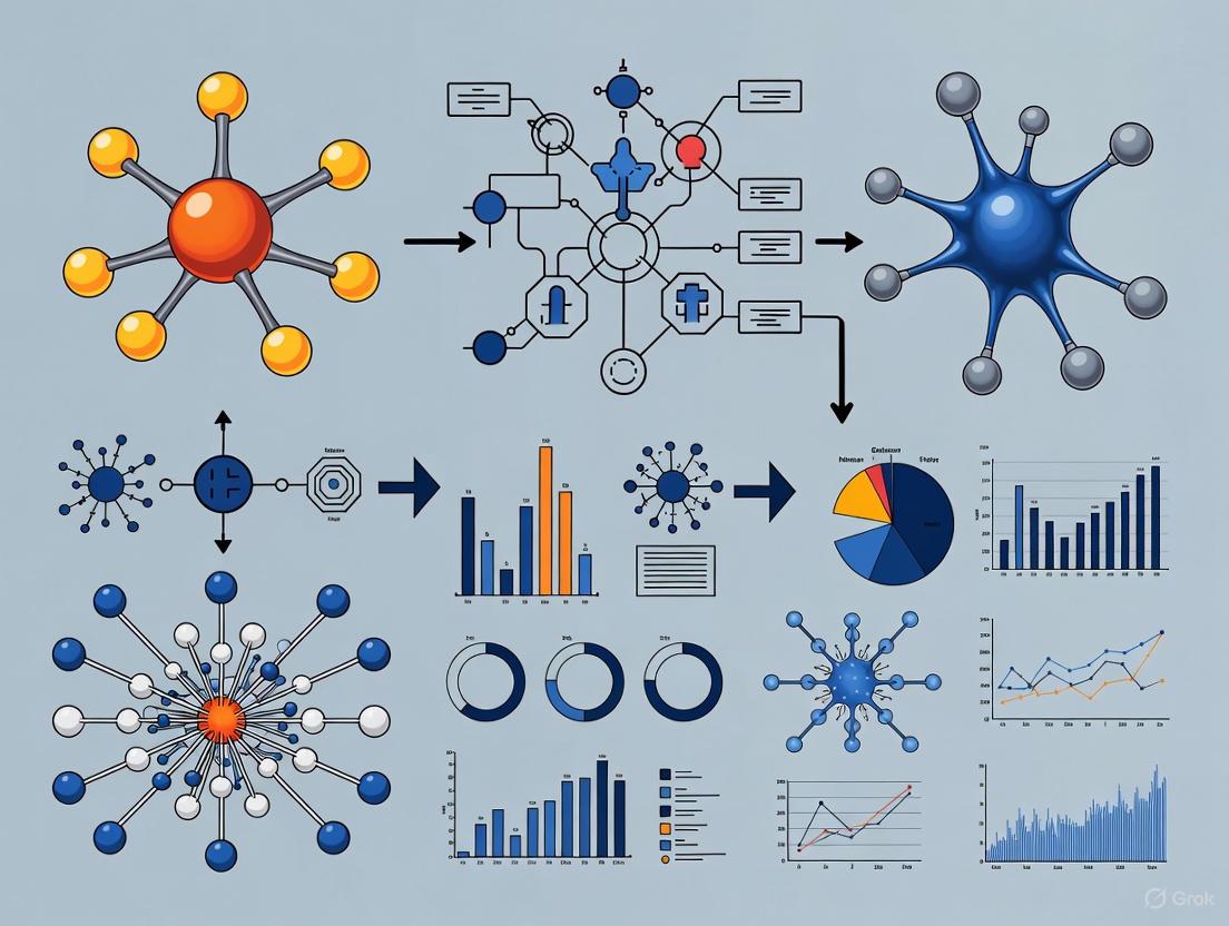
Diagnostic Diagrams

Diagram 1: The Domain Shift Problem in Neurotechnology

Diagram 2: A Framework for Cross-Subject Generalization

Theoretical Foundation: Why Brain Signals Inherently Cause Dataset Shift

What is the fundamental link between brain signal non-stationarity and dataset shift? Electroencephalography (EEG) and other brain signals are fundamentally non-stationary, meaning their statistical properties (like mean and variance) change over time [5] [6]. This inherent non-stationarity is a primary root cause of Dataset Shift in brain-computer interface (BCI) and neural decoder research [2]. When the data distribution changes between your training and testing environments, your model's performance degrades.

Aren't brain signals just noisy? Why can't we use standard linear methods? Brain signals are not just noisy; they are "3N" signals: Nonstationary, Nonlinear, and Noisy [5]. Using linear analysis methods (like FFT) on sufficiently long time intervals is inappropriate for such complex signals. The brain is a complex nonlinear system, and treating its signals as linear is a fundamental misunderstanding, akin to a geographer insisting the Earth is flat because their local measurements seem to form a plane [5].

Table: Core Properties of Brain Signals that Cause Dataset Shift

Property	Description	Consequence for Neural Decoders
Non-Stationarity [5] [2]	Statistical properties change over time due to switching between metastable brain states.	Models trained on data from one time session fail on data from another session.
Non-Linearity [5]	The output is not proportional to the input, and does not obey superposition principles.	Linear models and analyses fail to capture the true underlying dynamics of the signal.
Subject Variability [7]	Major inter-subject differences in neural morphology and signal patterns.	A model perfect for one subject performs poorly on another without adaptation.

Troubleshooting Guide: FAQs on Identifying and Solving Dataset Shift

FAQ 1: My model works perfectly in the lab but fails with new subjects. What happened?

You are likely experiencing Covariate Shift, a type of dataset shift where the distribution of input features (the EEG patterns) differs between your training lab subjects and new test subjects [8].

• Root Cause: The training data does not adequately represent the operating environment. This is often due to Sample Selection Bias during data collection or the inherent non-stationary environments of biological systems [8].
• Symptoms:
  • High accuracy during cross-validation on your original dataset.
  • Drastic drop in performance when the model is applied to data from a new session or a new subject.
• Solution:
  • Apply Transfer Learning: Use techniques like domain adaptation to align the feature distributions of your source (training) and target (new subject) data [2].
  • Utilize Subject-Invariant Features: Focus your feature engineering on discovering patterns that are robust across individuals [7].
  • Lightweight Calibration: Incorporate a small amount of data (e.g., 10%) from the new subject for calibration. Research has shown this can significantly boost performance (e.g., achieving accuracy of 0.781 and AUC of 0.801) [9].

FAQ 2: My decoder's performance drops over time, even for the same subject. How do I fix this?

This indicates Concept Drift, where the underlying relationship between the neural signals (input) and the decoded variable (output) has changed over time [8].

• Root Cause: The non-stationary nature of the brain means that the neural representations for the same task or state are not constant across sessions [5] [10].
• Symptoms:
  • Gradual degradation of model performance over multiple recording sessions.
  • The model becomes less reliable the longer it is in use.
• Solution:
  • Generative Models for Data Augmentation: Train a generative model (e.g., a Generative Adversarial Network or GAN) on an initial session. This model can then be rapidly adapted to new sessions with limited data to synthesize realistic new spike trains, effectively augmenting your training data and improving the decoder's robustness [10].
  • Continuous Learning Strategies: Implement algorithms designed for non-stationary data streams. Techniques like ELR (Effective Learning Rate) re-warming can help the model "unlearn" outdated features and adapt to new ones by periodically increasing the learning dynamics [11].
  • Session-Specific Calibration: Plan for regular, short re-calibration sessions to update the model parameters.

FAQ 3: How can I proactively test for dataset shift in my experimental pipeline?

Proactive detection is key to building robust models.

• Method: Statistical Distance Measures: Use metrics like the Kullback-Leibler (KL) divergence or Maximum Mean Discrepancy (MMD) to compare the probability distributions of your training data and your test (or deployment) data [8]. A large statistical distance is a clear warning sign of potential dataset shift.
• Method: Monitor Performance Metrics: Closely track metrics like loss and accuracy on a held-out validation set that is representative of your target deployment environment (e.g., containing multiple subjects). A growing gap between training and validation performance is a classic indicator of shift [8].

Table: Summary of Dataset Shift Types and Mitigation Strategies

Type of Shift	Definition	Best Mitigation Strategies
Covariate Shift [8]	The distribution of input features (X) changes between training and test.	- Domain Adaptation [2]- Importance Weighting- Subject-Invariant Representations [7]
Prior Probability Shift [8]	The distribution of the target variable (Y) changes.	- Adjusting classification thresholds.- Re-sampling training data.
Concept Drift [8]	The relationship between the inputs and outputs (X → Y) changes.	- Continuous Learning/Adaptation [11]- Generative models for data augmentation [10]- Regular model re-calibration.
Internal Covariate Shift	The distribution of inputs to hidden layers in a deep network changes during training.	- Use of Batch Normalization layers [8].

Experimental Protocols for Robust Generalization

Protocol: Cyclic Inter-Subject Training for Cross-Subject Generalization

This protocol is designed to learn a robust, subject-invariant initial model.

Objective: To create a neural decoder that generalizes well to unseen subjects by reducing primacy bias and encouraging feature learning [9] [11].

Workflow:

Methodology:

• Data Preparation: Pool data from multiple (N) source subjects.
• Cyclic Training: Instead of training on each subject's data sequentially to completion, the model is trained by alternating between subjects in short segments. For example, the model might be trained on a few batches from Subject 1, then a few batches from Subject 2, and so on, repeating this cycle [9].
• Outcome: This approach prevents the model from over-specializing on the first subject it sees (primacy bias) and encourages the development of generalized features that are useful across all subjects [11].

Protocol: Generative Model Adaptation for Cross-Session Decoding

This protocol uses a data-driven approach to tackle session-to-session variability.

Objective: To rapidly adapt a decoder to a new recording session or a new subject using only a small amount of new data [10].

Workflow:

Methodology:

• Base Model Training: A deep-learning generative model (e.g., a GAN) is trained on a full dataset from one source session. It learns a mapping from behavioral variables (e.g., hand kinematics) to the associated neural spike trains [10].
• Rapid Adaptation: The pre-trained generative model is then fine-tuned on a very small amount of data (as little as 35 seconds) from a new target session or subject.
• Data Augmentation: The adapted model synthesizes a virtually unlimited number of new, realistic neural data points that emulate the properties of the new session.
• Decoder Training: The BCI decoder is trained on a combination of the limited real data and the large volume of synthesized data. This augmented dataset leads to a more robust and better-generalizing decoder than training on the limited data alone [10].

The Scientist's Toolkit: Key Research Reagents & Materials

Table: Essential Resources for Cross-Subject/Session EEG Research

Resource / Reagent	Function / Application	Relevance to Generalization
HBN-EEG Dataset [7]	A large-scale public dataset with >3000 participants across 6 cognitive tasks.	Provides a benchmark for evaluating cross-task and cross-subject generalization.
Batch Normalization [8]	A layer in deep neural networks that standardizes its inputs.	Mitigates Internal Covariate Shift by stabilizing the distribution of inputs to hidden layers, accelerating training and improving performance.
Effective Learning Rate (ELR) Re-warming [11]	A training procedure that periodically increases the effective step size.	Counters primacy bias and loss of plasticity, helping models adapt to new data distributions in non-stationary environments.
Generative Adversarial Networks (GANs) [10]	A class of deep generative models that can learn to synthesize realistic data.	Used to create generative spike synthesizers for data augmentation, enabling robust decoder training with limited session-specific data.
Domain Adaptation Algorithms [2]	A suite of transfer learning methods designed to align feature distributions.	Directly addresses Covariate Shift by minimizing the discrepancy between source (training) and target (test) domains.

A fundamental challenge in modern neuroscience and brain-computer interface (BCI) research lies in the significant variability between individuals. Every brain is unique, with its structural and functional organization shaped by genetic and environmental factors over the course of development [12]. This individuality directly translates into inter-subject variability in the location of functional brain areas and the network organization of structural connectivity [12]. For neural decoders—computational models that map brain signals to stimuli or behavior—this variability poses a major obstacle. Models that perform well for one subject often fail when applied to another, or even on the same subject in a different recording session [10]. This technical support center addresses the core experimental and computational issues in achieving robust cross-subject and cross-session generalization for neural decoders, providing troubleshooting guides and methodologies for researchers and drug development professionals.

FAQs: Core Concepts in Neural Alignment & Generalization

1. What are brain-network alignment and neural tracking, and why are they critical for cross-subject generalization?

• Brain-Network Alignment refers to the process of establishing a meaningful correspondence between the neural nodes (e.g., brain regions) or network features of different individuals. It is necessary because the structural and functional properties of a specific region in a standard brain atlas are not perfectly equivalent across subjects [12]. Without proper alignment, comparing or aggregating neural data across subjects is invalid.
• Neural Tracking is the phenomenon where cortical activity automatically follows the dynamics of external stimuli, such as the acoustic or linguistic features of speech [13]. It ensures the temporal alignment of brain recordings with the stimuli or behavior they represent, providing a coherent signal for decoders to learn from.
• Together, they are foundational for generalization. Proper alignment ensures the decoder receives spatially comparable inputs across subjects, while neural tracking provides a temporally stable and consistent signal, enabling the model to learn universal mapping rules rather than subject-specific noise.

2. My subject-specific neural decoder performs well, but fails on new subjects. What is the primary cause?

The primary cause is the misalignment of feature spaces between subjects. Your decoder has likely learned features that are specific to the individual's neuroanatomy, electrode placement, or recording session characteristics. When applied to a new subject, these features are no longer relevant. This can be caused by:

• Structural misalignment: Differences in brain anatomy and parcellation mean that the same atlas region may contain functionally different neuronal populations across subjects [12].
• Functional misalignment: Even aligned regions may have different tuning properties or represent information in distinct ways [10].
• Signal property shifts: Differences in signal-to-noise ratio (SNR), electrode impedance, or recording hardware can alter the input distribution to the decoder [13].

3. What data-driven approaches can improve alignment without requiring extensive new data for each subject?

Recent advances leverage unsupervised and generative models:

• Graph Matching: This technique aligns the structural connectomes of different subjects by finding a permutation of the nodes (brain regions) of one graph that minimizes its dissimilarity to another. Using spatial adjacency as a prior in this process has been shown to effectively reduce inter-subject variability [12].
• Generative Adversarial Networks (GANs): A spike-train synthesizer can be trained on data from one session or subject and then rapidly adapted to a new subject using a small amount of data (e.g., 35 seconds). This model can then generate a virtually unlimited amount of realistic, subject-specific neural data to augment the training of a decoder, significantly improving its performance and generalization [10].
• Unified Models: Architectures like UniBrain are designed from the ground up to be subject-invariant. They use techniques like voxel aggregation to handle variable fMRI signal lengths and adversarial training with a subject discriminator to force the extraction of subject-invariant features, enabling zero-shot decoding on unseen subjects [14].

Troubleshooting Guides: From Theory to Practice

Problem 1: Poor Cross-Subject Decoding Performance

Symptoms: High performance on training subjects, but a significant drop in accuracy when the model is applied to held-out subjects.

Diagnosis and Solutions:

Potential Cause	Diagnostic Checks	Recommended Solution
Structural Misalignment	Check if node permutations from graph matching are largely non-identity [12].	Apply an unsupervised graph matching algorithm (e.g., FAQ) with spatial adjacency initialization to align subject connectomes before decoder training [12].
Subject-Specific Overfitting	Evaluate if your model uses subject-specific parameters or modules [14].	Transition to a unified model architecture (e.g., UniBrain) that uses adversarial feature alignment to learn subject-invariant representations [14].
Insufficient/Imbalanced Data	Analyze performance as a function of training set size for new subjects.	Use a generative model (e.g., GAN-based spike synthesizer) pre-trained on a source subject and adapted with minimal data from the target subject to augment your dataset [10].
Incorrect Input Assumptions	Verify if the model assumes fixed-length fMRI inputs across subjects [14].	Implement a group-based extractor that aggregates variable-length voxels into a fixed number of functionally coherent groups to standardize input size [14].

Problem 2: Unstable Performance Across Recording Sessions

Symptoms: Decoder accuracy degrades over time for the same subject, or varies significantly between sessions.

Diagnosis and Solutions:

Potential Cause	Diagnostic Checks	Recommended Solution
Neural Attribute Shift	Compare firing rates, tuning curves, or position activity maps between sessions [10].	Employ the same generative model adaptation strategy used for cross-subject generalization to rapidly recalibrate the decoder to the new session's neural attributes [10].
Changed Electrode Properties	Inspect signal impedance and noise levels.	Incorporate a domain adaptation layer that is trained to be invariant to session-specific signal properties [10].
Neural Plasticity	Check for gradual performance decline over long periods.	Implement a continuous learning framework that allows the decoder to slowly adapt to long-term changes without catastrophic forgetting of its original function.

Experimental Protocols for Validation

Protocol 1: Validating Cross-Subject Alignment with Graph Matching

Objective: To quantify and reduce the misalignment of structural connectomes across a group of subjects.

• Data Preparation: Obtain structural connectivity matrices for all subjects derived from the same parcellation atlas [12].
• Algorithm Selection: Choose a graph matching algorithm such as the Fast Approximate Quadratic (FAQ) algorithm, known to be effective for brain connectivity networks [12].
• Initialization: Initialize the algorithm with a Spatial Adjacency prior, which has been shown to outperform random or identity initialization by encouraging biologically plausible, local permutations [12].
• Alignment: For each subject pair, compute the permutation matrix ( P{ij} ) that minimizes the Frobenius norm ( \min{P \in \mathcal{P}} \lVert Gi - P^T Gj P \rVertF ), where ( Gi ) and ( G_j ) are the adjacency matrices [12].
• Validation:
  • Quantitative: Measure the reduction in the average Frobenius norm between subject connectomes after alignment. A significant decrease confirms improved group-wise similarity [12].
  • Qualitative: Characterize the obtained permutations. Successful alignment typically involves permutations between neighboring parcels, not distant brain areas [12].

Protocol 2: Evaluating Generalization with a Unified Model

Objective: To train and evaluate a neural decoder that generalizes to unseen subjects without subject-specific parameters.

• Model Architecture: Implement the UniBrain framework or similar [14]:
  • Group-Based Extractor: Aggregate variable-length fMRI voxels into a fixed number of groups based on functional similarity.
  • Mutual Assistance Embedder: A transformer-based module that decodes fMRI representations into both semantic and geometric embeddings in a coarse-to-fine manner.
  • Bilevel Feature Alignment: Use adversarial training at the extractor level and CLIP-space alignment at the embedder level to enforce subject invariance.
• Training Regime:
  • Train the model on data from a set of seen subjects.
  • Critical Step: Do not use any subject-specific parameters or modules [14].
• Evaluation:
  • In-Distribution (ID): Test on held-out data from the seen subjects. Performance should be comparable to state-of-the-art subject-specific models [14].
  • Out-of-Distribution (OOD): Test the model in a zero-shot manner on completely unseen subjects. This is the true test of cross-subject generalization. Report standard metrics like SSIM for image reconstruction or accuracy for classification tasks [14].

Essential Visualizations

Diagram 1: Cross-Subject Neural Decoding Workflow

Diagram 2: Bilevel Feature Alignment in Unified Models

The Scientist's Toolkit: Research Reagent Solutions

The following table details key computational and methodological "reagents" essential for experiments in cross-subject neural decoding.

Research Solution	Function & Application	Key Characteristics
Graph Matching Algorithms (e.g., FAQ) [12]	Aligns the nodes of structural or functional connectomes from different subjects to a common reference.	Reduces inter-subject variability; Improves similarity when parcels >100; Works best with spatial priors.
Generative Adversarial Networks (GANs) [10]	Synthesizes realistic neural spike trains; used for data augmentation and rapid adaptation to new subjects/sessions.	Captures neural attributes (tuning curves, firing rates); Enables adaptation with minimal data (e.g., 35 sec).
Unified Model Frameworks (e.g., UniBrain) [14]	A single model for all subjects that eliminates subject-specific parameters for zero-shot generalization.	Uses voxel aggregation and adversarial alignment; Drastically reduces parameter count; Enables OOD decoding.
Adversarial Feature Alignment [14]	A training scheme that forces the feature extractor to learn representations that a discriminator cannot use to identify the subject.	Creates subject-invariant features; Core component for preventing overfitting to subject-specific patterns.
Mutual Assistance Embedder [14]	Decodes neural representations into both semantic and geometric embeddings, which assist each other for richer reconstruction.	Coarse-to-fine decoding; Aligns with CLIP text and image features; Improves guidance for stimulus reconstruction.

This technical support center addresses common challenges in cross-subject and cross-session generalization for neural decoders, providing actionable guides for researchers and scientists.

Frequently Asked Questions

Q1: Why do my neural decoding models fail when applied to new subjects? Model failure on new subjects is primarily due to inter-subject variability [2] [15]. EEG and fMRI signals exhibit substantial individual differences caused by anatomical, physiological, and cognitive factors. This non-stationarity leads to the Dataset Shift problem, where the data distribution differs between training and deployment environments [2]. To address this, employ subject-invariant feature learning methods such as adversarial training [16] or contrastive learning [15] that explicitly disentangle subject-specific noise from semantic content.

Q2: What is the difference between cross-session and cross-subject generalization?

• Cross-Session Generalization: Focuses on maintaining performance for the same subject across different recording sessions, combating within-subject signal non-stationarity [2].
• Cross-Subject Generalization: Aims to decode neural data from completely new subjects not seen during training, requiring models to handle much larger inter-individual variability [2] [1]. Cross-subject scenarios are generally more challenging but essential for scalable BCI systems.

Q3: How can I achieve decent performance with minimal data from new subjects? Few-shot calibration is highly effective. Research shows that incorporating just 10% of a target subject's data for calibration can achieve an accuracy of 0.781 and AUC of 0.801 in imagined speech detection tasks [9]. Implement cyclic inter-subject training with shorter per-subject segments and frequent alternation among subjects during pretraining to build a robust base model [9].

Q4: What methods work best for zero-shot cross-subject decoding? For true zero-shot scenarios (no target subject data), the most promising approaches include:

• Explicit feature disentanglement to separate subject-related and semantic-related components [16]
• Adversarial training to learn subject-invariant representations [16]
• Contrastive learning in hyperbolic space to capture hierarchical relationships in neural data [15]
• Functional alignment techniques like ridge regression or hyperalignment to map subjects to a common space [17]

Q5: How do I choose between functional and anatomical alignment?

• Anatomical Alignment: Transforms individual brains to match a standard template using anatomical landmarks. Effective for larger brain structures but may lack precision for smaller, variable regions [17].
• Functional Alignment: Synchronizes brain activity patterns across individuals. Ridge regression has emerged as superior for fine-grained information decoding, outperforming other functional alignment techniques in cross-subject brain decoding studies [17].

Use functional alignment when dealing with high-level cognitive tasks or when precise functional localization is critical. Anatomical alignment suffices for basic spatial normalization.

Troubleshooting Guides

Problem: Poor Cross-Subject Generalization in EEG Emotion Recognition

Symptoms: Model performs well on training subjects but accuracy drops significantly (15-30%) on new subjects.

Solutions:

• Implement Cross-Subject Contrastive Learning (CSCL)
  • Employ dual contrastive objectives with emotion and stimulus contrastive losses
  • Use hyperbolic space instead of Euclidean to better capture hierarchical relationships
  • Implement a triple-path encoder integrating spatial, temporal, and frequency information [15]

• Apply Dynamic Brain Functional Networks
  • Construct time-varying functional connectivity using sliding windows
  • Extract network attributes: global efficiency, local efficiency, and local clustering coefficients
  • This approach achieved 91.17% accuracy in arousal classification on DEAP dataset [18]

Verification: Test on multiple benchmark datasets (SEED, DEAP, MPED) to ensure robustness. Cross-subject contrastive learning has shown 97.70% accuracy on SEED, 96.26% on CEED, and 65.98% on FACED datasets [15].

Problem: Limited Cross-Task Generalization

Symptoms: Model trained on one cognitive task (e.g., motor imagery) fails to decode other tasks (e.g., emotion recognition).

Solutions:

• Utilize Foundation Model Approaches
  • Train on massive, diverse datasets encompassing multiple tasks and subjects
  • The EEG Foundation Challenge uses 3,000+ subjects with six distinct cognitive tasks [1]
  • Implement architectures capable of learning domain-invariant and subject-invariant representations [1]

• Adopt Unified Frameworks
  • NEED framework achieves cross-task generalization for both video and image reconstruction from EEG
  • Uses Individual Adaptation Module pretrained on multiple EEG datasets [4]
  • Implements dual-pathway architecture capturing both low-level visual dynamics and high-level semantics [4]

Verification: Evaluate using zero-shot cross-task benchmarks. Successful models maintain 93.7% of within-subject classification performance when transferring to unseen tasks [4].

Problem: Subject-Specific Noise Overwhelming Semantic Content

Symptoms: Model learns to identify subjects rather than neural content, failing to extract task-relevant information.

Solutions:

• Apply Explicit Disentanglement Framework
  • Use Zebra's four-component decomposition: subject-invariant, subject-specific, semantic-specific, and semantically irrelevant features [16]
  • Implement residual decomposition and adversarial training to remove subject-specific noise [16]
  • Project semantic-specific features into shared visual-semantic space aligned with CLIP embeddings [16]

• Leverage Multi-Subject Training with Alignment
  • Align multiple subjects using ridge regression, which outperforms hyperalignment in fine-grained decoding [17]
  • Train on one subject, align new subjects to this space, enabling cross-subject decoding with 90% reduction in required scan time [17]

Verification: Quantitative metrics should show significant improvement in semantic-relevant metrics (e.g., +0.084 PixCorr gain) while reducing subject identification accuracy.

Performance Comparison Tables

Table 1: Cross-Subject Emotion Recognition Performance Across Methods

Method	Dataset	Accuracy	Key Innovation
CSCL (Contrastive Learning) [15]	SEED	97.70%	Hyperbolic space, triple-path encoder
CSCL (Contrastive Learning) [15]	CEED	96.26%	Emotion and stimulus contrastive losses
CSCL (Contrastive Learning) [15]	FACED	65.98%	Region-aware learning mechanism
Dynamic Brain Network [18]	DEAP (Arousal)	91.17%	Time-varying functional connectivity
Dynamic Brain Network [18]	DEAP (Valence)	90.89%	Network attribute features
MdGCNN-TL [18]	DEAP	65.89%	Graph neural network with transfer learning
MSRN+MTL [18]	DEAP	71.29%	Multi-scale residual network

Table 2: Zero-Shot Cross-Subject Decoding Performance

Method	Modality	Task	Performance vs. Fine-Tuned	Key Metric
Zebra [16]	fMRI	Visual Decoding	Comparable to fully fine-tuned	SSIM: 0.384 (vs. 0.375 fine-tuned)
Zebra [16]	fMRI	Visual Decoding	+0.084 PixCorr gain	0.153 vs. 0.069 baseline
NEED [4]	EEG	Video Reconstruction	92.4% of within-subject quality	Cross-task SSIM: 0.352
Ridge Regression Alignment [17]	fMRI	Image Reconstruction	90% scan time reduction	Comparable to single-subject decoding

Experimental Protocols

Protocol 1: Cross-Subject Contrastive Learning for EEG Emotion Recognition

This protocol implements the CSCL framework for robust cross-subject emotion recognition [15].

Materials:

• EEG recording system (128-channel recommended)
• Emotional stimulus presentation setup
• Standard preprocessing pipeline (filtering, artifact removal)

Procedure:

• Data Preparation:
  • Extract segments from EEG signals during emotional stimulus presentation
  • Apply standard preprocessing: bandpass filtering, artifact removal
  • Normalize data per subject

• Feature Extraction:

  • Implement triple-path encoder:
    • Spectral Path: Compute frequency-domain features (PSD, DE)
    • Temporal Path: Extract time-domain patterns
    • Spatial Path: Model inter-channel relationships
  • Combine features using attention-based fusion

• Contrastive Learning:

  • Project features into hyperbolic space using Poincaré embeddings
  • Apply dual contrastive losses:
    • Emotion Contrastive Loss: Pull same emotion classes together, push different apart
    • Stimulus Contrastive Loss: Maintain consistency across same stimuli
  • Optimize using Riemannian optimization methods

• Classification:

  • Use simple classifier (MLP) on learned representations
  • Evaluate using leave-one-subject-out cross-validation

Validation: Test on multiple datasets (SEED, CEED, FACED, MPED) to ensure generalizability.

Protocol 2: Zero-Shot fMRI Visual Decoding with Disentanglement

This protocol implements the Zebra framework for zero-shot cross-subject visual decoding [16].

Materials:

• fMRI data (7T recommended for visual decoding)
• Visual stimulus set (natural images)
• Pretrained ViT and CLIP models

Procedure:

• Data Preprocessing:
  • Convert fMRI data to 2D brain activation maps (256×256)
  • Apply anatomical alignment to standard space
  • Extract region-of-interest (especially visual cortex)

• Subject-Invariant Feature Extraction:

  • Use ViT-based fMRI encoder (fMRI-PTE) pretrained on multi-subject data
  • Apply adversarial training with gradient reversal
  • Implement residual decomposition to separate subject-specific variations

• Semantic-Specific Feature Learning:

  • Project features to CLIP space using diffusion prior
  • Align with visual embeddings using contrastive loss
  • Preserve semantic discriminability while removing subject information

• Image Reconstruction:

  • Use diffusion model for image generation from semantic embeddings
  • Employ pre-trained Stable Diffusion with guided sampling
  • Generate reconstructions from subject-invariant features only

Validation Metrics:

• Structural Similarity (SSIM)
• Pixel Correlation (PixCorr)
• AlexNet(5) accuracy for semantic content
• Subject identification accuracy (should be at chance level)

Research Reagent Solutions

Table 3: Essential Tools for Neural Decoding Research

Tool	Function	Example Use Cases
fMRI-PTE [16]	ViT-based fMRI encoder	Mapping fMRI to unified 2D representations
Dynamic Brain Networks [18]	Time-varying connectivity analysis	Capturing evolving neural patterns in emotion
CLIP Embeddings [16]	Semantic feature alignment	Bridging neural and visual semantic spaces
Hyperbolic Embeddings [15]	Hierarchical representation learning	Modeling complex relationships in neural data
Diffusion Prior [16]	Latent space transformation	Converting neural to visual embeddings
Adversarial Discriminators [16]	Subject-invariant learning	Removing subject-specific noise
Contrastive Loss Functions [15]	Representation enhancement	Learning invariant emotional features

Methodological Diagrams

Diagram 1: Cross-Subject Generalization Framework

Diagram 2: Zero-Shot Disentanglement Pipeline

Diagram 3: Contrastive Learning for EEG Emotion Recognition

The Impact of Theoretical Models and Participant Screening on Decoder Performance

Troubleshooting Guides

FAQ 1: Why does my neural decoder perform poorly on new subjects, and how can I fix it?

Issue: A model trained on one set of subjects shows significantly degraded performance (e.g., lower classification accuracy or reconstruction quality) when applied to new, unseen subjects. This is a classic problem of poor cross-subject generalization.

Explanation: A primary cause is the high degree of inter-subject variability in brain anatomy and functional organization. Decoders often learn to rely on subject-specific neural patterns that do not transfer well. Furthermore, if the training data lacks sufficient subject diversity, the model fails to learn the underlying, invariant neural code.

Solutions:

• Adversarial Disentanglement: Implement frameworks like ZEBRA, which use adversarial training to explicitly disentangle fMRI representations into subject-related and semantic-related components. This forces the model to isolate subject-invariant features, enabling zero-shot generalization to new subjects without fine-tuning [19].
• Input Normalization: Employ an Individual Adaptation Module, pre-trained on multiple datasets, to help normalize subject-specific patterns in EEG data before the main decoding stage. This has been shown to maintain over 92% of visual reconstruction quality on unseen subjects [4].
• Multi-Subject Pretraining: Pretrain your model on data from a large number of subjects across diverse tasks. As demonstrated with transformer models on calcium imaging data, combining data from different sources builds more robust representations that can transfer to new subjects and even new brain regions [20].

FAQ 2: How can I improve my decoder's generalization across different tasks or experimental sessions?

Issue: A decoder trained for one specific cognitive task (e.g., listening to speech) fails to perform well on a different but related task (e.g., reading), limiting its practical utility.

Explanation: Models can become overly specialized to the statistical regularities of a single task or session. Variations in cognitive state, attention, and low-level sensory processing between tasks and sessions can render these models ineffective.

Solutions:

• Multi-Task Pretraining: Train a single model on multiple tasks simultaneously. Research on multi-task transformers shows that this approach allows the model to extract common information from diverse neural circuits, facilitating transfer to new tasks and sessions [20].
• Unified Architecture: Design a model with a flexible inference mechanism that can adapt to different visual or cognitive domains. The NEED framework, for example, uses a dual-pathway architecture to capture both low-level visual dynamics and high-level semantics, allowing it to handle both video and image reconstruction from EEG without task-specific fine-tuning [4].
• Leverage Foundation Models: Utilize large, pre-trained models, such as Large Language Models (LLMs), as a backbone. Their powerful, general-purpose representations of information can be aligned with neural activity, providing a strong prior that improves generalization to new tasks and contexts [13].

FAQ 3: My decoder works in offline analysis but is too slow for real-time use. How can I optimize for speed?

Issue: The model achieves good accuracy but has high latency and computational demands, making it unsuitable for real-time brain-computer interface (BCI) applications or closed-loop experiments.

Explanation: Complex architectures like Transformers, while accurate, often have significant computational overhead. The choice of model architecture and compiler settings directly impacts inference speed.

Solutions:

• Hybrid Architecture: Use a hybrid model like POSSM, which combines a recurrent State-Space Model (SSM) backbone with a cross-attention module for spike tokenization. This architecture is designed for causal, online prediction and has been shown to achieve accuracy comparable to Transformers while being up to 9x faster on GPU [21].
• Compiler and Precision Tuning: Utilize compiler flags to optimize the trade-off between speed and accuracy. For instance, on AWS Neuron, using the --auto-cast flag can improve performance by using lower precision (BF16), though this may sometimes affect accuracy and requires careful validation [22].
• Model Warmup: For consistent low-latency inference, ensure the model is properly "warmed up" before processing critical requests. This can be done by sending a few dummy prompts through the system to initialize states and caches, mitigating slow initial responses [22].

FAQ 4: What is the impact of data preprocessing on decoder performance and generalization?

Issue: Decoding performance is highly sensitive to the specific preprocessing pipeline applied to the raw neural data (e.g., EEG), making results difficult to reproduce and generalize.

Explanation: Preprocessing steps directly shape the input features the decoder learns from. Certain steps may remove biologically relevant signals or, conversely, leave in structured noise that the model can exploit, leading to inflated but non-generalizable performance.

Solutions:

• Systematic Pipeline Evaluation: Adopt a "multiverse" approach, where you systematically test multiple preprocessing paths. One study varied filtering, artifact correction, and referencing, finding that choices like high-pass filter cutoff significantly influenced decoding accuracy [23].
• Caution with Artifacts: Be aware that artifact correction steps (e.g., ICA for ocular artifacts) can sometimes reduce decoding performance because the artifacts themselves may be systematically correlated with the task (e.g., eye movements in a visual attention task). The decision to correct must balance performance against the interpretability of the neural signal [23].
• Use Sensible Defaults: Start with established preprocessing defaults for your modality. For example, the study recommends using higher high-pass filter cutoffs and linear detrending, which consistently boosted decoding performance across multiple EEG experiments [23].

Experimental Protocols & Data

Key Experiment: Evaluating Preprocessing Choices

Objective: To quantitatively assess how different EEG preprocessing steps influence cross-subject decoding performance.

Methodology:

• Data: Use a publicly available dataset (e.g., ERP CORE) containing multiple experiments and participants [23].
• Multiverse Design: Systematically vary key preprocessing steps to create a "multiverse" of analysis pipelines. The steps should include:
  • High-pass and low-pass filter cutoffs
  • Artifact correction methods (ICA for ocular/muscle artifacts, Autoreject)
  • Reference scheme (e.g., average, Cz)
  • Baseline correction and detrending
• Decoding: Train and evaluate a decoder (e.g., EEGNet or time-resolved logistic regression) for each preprocessing path on each subject.
• Analysis: Use linear mixed models to estimate the marginal effect of each preprocessing step on decoding performance, isolating its impact from other steps.

Key Quantitative Findings: The table below summarizes the average impact of specific preprocessing choices on decoding performance across several EEG experiments [23].

Table: Impact of EEG Preprocessing Steps on Decoding Performance

Preprocessing Step	Option A	Effect on Performance	Option B	Effect on Performance
High-Pass Filter	Lower Cutoff (0.01 Hz)	↓ Decrease	Higher Cutoff (0.1-1 Hz)	↑ Increase
Low-Pass Filter	Lower Cutoff (20 Hz)	↑ Increase (Time-resolved)	Higher Cutoff (40 Hz)	Mixed / Neutral
Ocular Artifact Correction	ICA Correction	↓ Decrease	No Correction	↑ Increase*
Muscle Artifact Correction	ICA Correction	↓ Decrease	No Correction	↑ Increase*
Detrending	Linear Detrending	↑ Increase	No Detrending	↓ Decrease
Baseline Correction	Longer Interval	↑ Increase	No / Short Interval	↓ Decrease

*Performance increase may come from decoding structured noise (e.g., eye movements) correlated with the task, reducing result interpretability [23].

Key Experiment: Adversarial Training for Cross-Subject Generalization

Objective: To enable a visual decoding model to perform accurately on fMRI data from unseen subjects without any subject-specific fine-tuning.

Methodology:

• Model Architecture (ZEBRA): Design a framework with a shared feature encoder followed by two branches:
  • A semantic decoder for reconstructing images from brain activity.
  • A subject discriminator that tries to predict the subject identity from the features.
• Adversarial Training: Train the model with a dual objective:
  • The semantic decoder minimizes reconstruction loss.
  • The feature encoder is trained to fool the subject discriminator, using a gradient reversal layer. This encourages the encoder to produce features that are informative for reconstruction but uninformative about subject identity [19].
• Evaluation: Test the model in a zero-shot setting on held-out subjects and compare performance against subject-specific models.

Diagrams & Workflows

Diagram: Adversarial Disentanglement for Cross-Subject Generalization

Diagram: Hybrid Model for Real-Time Decoding

The Scientist's Toolkit: Research Reagent Solutions

Table: Essential Tools and Methods for Neural Decoding Research

Research Reagent / Method	Function & Explanation
Adversarial Training	A learning technique used to disentangle latent representations. It helps create subject-invariant features by forcing the model to fool a subject-classifier, improving cross-subject generalization [19].
State-Space Models (SSMs)	A class of recurrent models known for efficient long-range sequence modeling. They form the backbone of hybrid architectures like POSSM, enabling fast, real-time neural decoding with low inference latency [21].
Multi-Task Transformers	A flexible architecture trained on diverse datasets and tasks. It allows for transfer learning between different brain regions, cell types, and cognitive tasks, building large-scale, generalizable models of neural activity [20].
Individual Adaptation Module	A pre-processing component designed to normalize subject-specific patterns in neural data (e.g., EEG). It acts as a subject "filter" to reduce inter-subject variability before the main decoding stage [4].
Multiverse Analysis	A systematic grid-search methodology for evaluating multiple analysis pipelines (e.g., preprocessing steps). It quantifies the impact of analytical choices on outcomes like decoding performance, improving robustness and reproducibility [23].

Building Robust Decoders: Architectures and Transfer Learning Strategies for Real-World Application

Frequently Asked Questions

Q1: Why does my neural decoder's performance degrade when used on a different subject or in a new session? This is a classic problem of Dataset Shift, primarily caused by the non-stationary, non-linear, and non-Gaussian nature of neural signals [24]. Brain electrical activity varies between individuals due to differences in electrode placement, tissue characteristics, and inherent neuronal activity patterns [24]. Even for the same subject, physiological states and electrode conditions change over time, leading to significant distributional differences in the data between sessions [24]. Conventional models trained under the assumption that data is independently and identically distributed fail under these cross-subject/session conditions [24].

Q2: What is the fundamental difference between conventional approaches and Domain Adaptation? Conventional machine learning approaches train a decoder for a specific subject or session. In contrast, Domain Adaptation is a transfer learning technique that leverages knowledge from a labeled source domain (e.g., data from previous subjects or sessions) to improve learning and performance in a different but related target domain (a new subject or session), even when their joint probability distributions differ [24]. The core objective is to learn a decision function for the target domain that minimizes prediction error by aligning the distributions between domains [24].

Q3: My model works well on the training data but fails on new subjects. Is this an overfitting problem? While overfitting can be a factor, the primary issue is often model generalizability. A systematic review of EEG-based emotion recognition confirms that standard models suffer from the dataset shift problem in cross-subject and cross-session scenarios [2]. Transfer learning and domain adaptation methods are specifically designed to overcome this by improving the generalization of models to new, unseen data domains [2].

Q4: How much source domain data is typically needed for effective transfer learning? While requirements vary, some benchmarks in related fields suggest that for time-series data, having more than three weeks of periodic data or a few hundred buckets for non-periodic data is a good rule of thumb [25]. For neural decoding, a large EEG dataset used for cross-session studies contained 5 sessions per subject with 100 trials each, providing a robust foundation for adaptation algorithms [26].

Troubleshooting Guides

Issue 1: Poor Cross-Subject Generalization

Symptoms: High accuracy for the subject used in training, but a significant performance drop when the decoder is applied to new subjects.

Step	Action	Technical Details
1. Diagnosis	Check for covariate shift between subjects.	Use dimensionality reduction (e.g., t-SNE, PCA) to visualize feature distributions from different subjects. If subject clusters are separate, domain shift is confirmed.
2. Solution	Apply Feature-Based Domain Adaptation [24].	Transform source and target domain features into a shared space where distributions are aligned. Common methods include Correlation Alignment (CORAL) or Maximum Mean Discrepancy (MMD) minimization [24].
3. Implementation	Use an adversarial learning framework.	Train a feature extractor to generate domain-invariant features that can fool a simultaneous domain classifier [24].
4. Validation	Perform cross-subject validation.	Strictly leave one subject out for testing and report average performance across all left-out subjects, never mixing subject data [2].

Issue 2: Cross-Session Performance Instability

Symptoms: Decoder performance decays over time, or a model trained on day one performs poorly on data from the same subject collected days or weeks later.

Step	Action	Technical Details
1. Diagnosis	Assess performance drop using benchmark metrics.	One study reported within-session accuracy of 68.8% dropping to cross-session accuracy of 53.7% without adaptation [26].
2. Solution	Implement Partial Domain Adaptation (PDA) [27].	PDA performs neural alignment only within the task-relevant latent subspace, disentangling it from task-irrelevant neural components that cause instability [27].
3. Implementation	Construct a causal dynamical system.	With pre-aligned short-time windows as input, use VAE-based representation learning and adversarial alignment to disentangle features [27].
4. Validation	Use Lyapunov theory.	Analytically validate the improved stability of the neural representations after alignment [27]. Experiments show PDA significantly enhances cross-session decoding performance [27].

Issue 3: Model Overfitting to Source Domain

Symptoms: The model performs excellently on the source domain data but fails to adapt to the target domain, even after fine-tuning.

Step	Action	Technical Details
1. Diagnosis	Check for overfitting during pre-training.	If the model is too complex or trained for too many epochs on the source data, it may learn features too specific to that domain.
2. Solution	Apply Instance-Based DA [24].	Strategically reduce the weights of labeled source domain samples that have a distribution significantly different from the target domain. This minimizes negative transfer [24].
3. Implementation	Sample weighting or selection.	Weight or select source domain samples based on their similarity to the target domain distribution before performing knowledge transfer [24].
4. Validation	Monitor target domain loss during fine-tuning.	A continuously high or increasing target domain loss indicates the model is struggling to adapt, possibly due to overfitting to the source.

Performance Data and Benchmarks

Table 1: Benchmarking Performance of Different Learning Paradigms in a Motor Imagery EEG Dataset [26]

Learning Paradigm	Description	Average Classification Accuracy
Within-Session (WS)	Model trained and tested on data from the same session.	68.8%
Cross-Session (CS)	Model trained on one session and tested on another without adaptation.	53.7% (Not significantly different from chance level)
Cross-Session Adaptation (CSA)	Model adapted using a small amount of target session data.	78.9%

Table 2: Categorization of Domain Adaptation Methods for Neural Decoding [24]

Method Category	Core Principle	Typical Algorithms	Best For
Instance-Based	Weight or select source samples similar to the target domain.	Sample weighting, importance sampling.	Scenarios where parts of the source data are still relevant.
Feature-Based	Transform features to align source and target distributions.	CORAL, MMD, Adversarial Alignment.	Bridging significant distributional gaps between subjects/sessions.
Model-Based	Fine-tune a pre-trained model on a small target dataset.	Parameter sharing, fine-tuning of pre-trained layers.	When labeled target data is scarce but a large source dataset exists.

Experimental Protocols for Validation

Protocol 1: Validating Cross-Subject Generalization

Objective: To evaluate how well a neural decoder trained on multiple subjects generalizes to a completely new subject.

Diagram: Cross-Subject Validation via Feature Alignment

• Data Partitioning: Reserve data from one or more subjects as the target domain. The remaining subjects form the source domain [2].
• Feature Alignment: Train a feature extractor to project data from both domains into a shared feature space where their distributions are aligned. This can be achieved by minimizing a divergence metric like MMD or through adversarial training [24].
• Decoder Training: Train the decoder model using the labeled data from the aligned source domain features.
• Validation: Test the final model on the held-out target subject's data. Repeat this process for all subjects (e.g., leave-one-subject-out cross-validation) [2].

Protocol 2: Validating Cross-Session Stability

Objective: To assess the long-term stability of a neural decoder and the effectiveness of adaptation techniques across different sessions.

Diagram: Cross-Session Stability with Partial Domain Adaptation

• Longitudinal Data Collection: Collect data from the same subject across multiple sessions, with intervals of days or weeks (e.g., a 5-session dataset over 10 days) [26].
• Base Model Pre-training: Train an initial model on data from the first session.
• Partial Domain Adaptation: When new session data arrives, employ a PDA framework. Use a causal dynamical system model to disentangle task-relevant neural features from task-irrelevant components. Perform adversarial alignment only on the task-relevant latent subspace [27].
• Stability Analysis: Use analytical tools like Lyapunov theory to validate the improved stability of the neural representations [27].
• Performance Tracking: Evaluate the adapted decoder on all subsequent sessions to monitor performance stability over time.

The Scientist's Toolkit: Research Reagent Solutions

Table 3: Essential Materials and Algorithms for Neural Decoding Research

Item / Solution	Function / Purpose	Example Use Case
Large Public Neuroimaging Datasets (e.g., HCP [28], OpenNeuro [28])	Provides extensive source domain data for pre-training deep learning models, which is crucial for transfer learning success.	Pre-training a whole-brain fMRI cognitive decoder on the Human Connectome Project dataset before fine-tuning on a smaller, study-specific dataset [28].
EEG Motor Imagery Datasets (e.g., 5-session cross-session dataset [26])	Offers benchmark data specifically designed for testing cross-session and cross-subject generalization.	Benchmarking a new domain adaptation algorithm against standard WS, CS, and CSA performance metrics [26].
Adversarial Alignment Frameworks	A feature-based DA method that uses a domain classifier to force the feature extractor to learn domain-invariant representations [24].	Creating a subject-invariant EEG feature space for emotion recognition, improving classifier performance on new subjects [24].
Partial Domain Adaptation (PDA)	A specialized DA framework that identifies and aligns only task-relevant neural components, ignoring task-irrelevant noise [27].	Achieving stable long-term decoding performance in BCI applications across different experimental days, countering non-stationarity [27].
Common Spatial Patterns (CSP) & Filter Bank CSP (FBCSP)	Classic spatial filtering algorithms for feature extraction in Motor Imagery BCI [26].	Used as a strong baseline feature extraction method before applying domain adaptation techniques [26].
Deep ConvNets / EEGNet	End-to-end deep learning models for neural signal decoding that can learn complex features directly from raw or pre-processed data [26].	Serving as a powerful backbone model that can be combined with DA techniques for improved end-to-end cross-subject decoding [24].

Q: What is the NEED framework and what core problem does it solve? A: The NEED framework is the first unified model designed for zero-shot cross-subject and cross-task generalization in EEG-based visual reconstruction. It addresses the critical limitations of poor generalization across subjects and constraints to specific visual tasks that have hindered previous neural decoding systems. NEED allows a single model to work on new subjects and different visual tasks (like video or static image reconstruction) without requiring any subject-specific data or retraining [4].

Q: What are the main architectural components of NEED that enable this generalization? A: NEED tackles generalization through three key innovations [4]:

• Individual Adaptation Module: Pretrained on multiple EEG datasets to normalize subject-specific neural patterns.
• Dual-Pathway Architecture: Captures both low-level visual dynamics and high-level semantic content from EEG signals.
• Unified Inference Mechanism: Allows the model to adapt to different visual domains (e.g., video and images) within a single framework.

Performance Data & Generalization Metrics

The table below summarizes the key quantitative results of the NEED framework as reported in the research, demonstrating its strong cross-subject and cross-task performance.

Table 1: NEED Framework Performance Metrics

Generalization Scenario	Metric	Performance	Significance
Cross-Subject (Unseen Subjects)	Retention of within-subject classification performance	93.7%	Model retains nearly all its classification capability on new subjects without fine-tuning [4].
Cross-Subject (Unseen Subjects)	Retention of visual reconstruction quality	92.4%	Reconstructed visuals for new subjects are nearly identical in quality to those for known subjects [4].
Cross-Task (Zero-shot transfer to static image reconstruction)	Structural Similarity Index (SSIM)	0.352	Demonstrates direct applicability to a new task (image reconstruction) without model retraining [4].

Experimental Protocols

Protocol 1: Validating Cross-Subject Generalization

This protocol outlines the steps to evaluate how well the NEED framework performs on EEG data from previously unseen subjects.

Table 2: Cross-Subject Validation Protocol

Step	Action	Purpose	Key Inputs
1.	Data Preparation	Ensure clean, standardized input data for the model.	Preprocessed EEG datasets from multiple subjects.
2.	Subject Splitting	Simulate a real-world scenario with new users.	Hold out one or more subjects' data for testing.
3.	Model Inference	Generate predictions for the unseen subject.	Trained NEED model; held-out subject's EEG data.
4.	Performance Quantification	Measure generalization capability objectively.	Compare reconstructed images/videos to ground truth using SSIM and classification accuracy [4].

Protocol 2: Zero-Shot Cross-Task Transfer

This protocol describes the methodology for applying the NEED framework to a new visual task, such as moving from video to static image reconstruction, without any task-specific fine-tuning.

Table 3: Cross-Task Validation Protocol

Step	Action	Purpose	Key Outputs
1.	Task Definition	Clearly define the new target domain.	Static image reconstruction stimuli and corresponding EEG data.
2.	Direct Inference	Assess inherent model flexibility.	NEED model trained only on video reconstruction tasks.
3.	Evaluation	Gauge quality of transfer.	SSIM score of 0.352 for image reconstruction, confirming effective zero-shot transfer [4].

Framework Architecture & Workflow

The following diagram illustrates the core architecture and data flow of the NEED framework, highlighting how it achieves cross-subject and cross-task generalization.

NEED Framework Core Architecture

The Scientist's Toolkit: Research Reagent Solutions

The table below lists key computational tools and methodological components essential for implementing and experimenting with generalized neural decoders like the NEED framework.

Table 4: Essential Research Reagents for Neural Decoding Generalization

Reagent / Method	Function	Application in NEED
Individual Adaptation Module (IAM)	Normalizes subject-specific patterns in neural data.	Isolates subject-invariant, semantic-specific EEG representations for cross-subject generalization [4].
Adversarial Training	A training technique where a generator and discriminator network compete.	Used to explicitly disentangle subject-related and semantic-related components of fMRI/EEG representations [19].
Dual-Pathway Architecture	A neural network structure that processes information through separate streams.	Captures both low-level visual dynamics and high-level semantics from EEG signals for robust feature extraction [4].
Generative Adversarial Networks (GANs)	A class of AI models that learn to generate new data with the same statistics as the training set.	Can be used as a generative spike-train synthesizer to create synthetic neural data for augmenting BCI decoder training and improving cross-session generalization [10].
Zero-Shot Learning	A paradigm where a model performs a task without having seen any example of that task during training.	The core of NEED's inference mechanism, allowing it to perform cross-task visual reconstruction (e.g., video to images) without fine-tuning [4].

Frequently Asked Questions (FAQs)

1. What is the primary advantage of using a Hilbert Transform over a Fourier Transform in neural decoding models? The Hilbert Transform (HT) provides two key advantages that are crucial for neural decoding. First, it creates an analytic signal that removes non-physical negative frequencies, preventing spectrum waste and undesirable artifacts caused by their interaction with positive frequencies [29]. Second, unlike the global analysis of Fourier Transform, HT enables time-frequency analysis, allowing the calculation of instantaneous frequency with a resolution that reaches the sampling resolution of the observed signal [29]. This provides more fine-grained temporal information about neural dynamics.

2. My HTNet model generalizes poorly across subjects. What strategies can improve cross-subject performance? Poor cross-subject generalization often stems from model overfitting to subject-specific neural patterns. To address this:

• Adversarial Disentanglement: Implement frameworks like ZEBRA, which use adversarial training to explicitly decompose fMRI representations into subject-related and semantic-related components. This isolates subject-invariant, semantic-specific features, enabling zero-shot generalization to unseen subjects [19].
• Leverage Large Language Models (LLMs): Integrate pre-trained LLMs for their powerful information understanding and processing capacities. Their representations account for a significant portion of the variance in human brain activity during language tasks, improving model robustness [13].
• Check Data Alignment: Ensure temporal alignment of brain recordings with linguistic representations. A minor time shift can disrupt the association between language stimuli and neural patterns, harming generalization [13].

3. How do brain-region projection layers in HTNet adapt to different behavioral states? Evidence suggests that prefrontal cortex (PFC) subregions send highly specialized, state-dependent signals to posterior brain regions. For instance, the orbitofrontal cortex (ORB) and anterior cingulate area (ACA) selectively transmit information about arousal and motion to the primary visual cortex (VISp). These signals dynamically sharpen or suppress visual information processing based on the subject's arousal level and whether it is moving, effectively balancing each other to enhance relevant stimuli and suppress irrelevant ones [30].

4. What are the key evaluation metrics for a neural decoding model like HTNet in a cross-subject context? The choice of metric depends on your specific decoding task. The table below summarizes the most relevant metrics [13].

Task Paradigm	Key Metric	Description
Stimuli Recognition	Accuracy	Percentage of correctly identified stimuli instances.
Brain Recording Translation	BLEU, ROUGE, BERTScore	Measures semantic consistency of decoded text with reference text; focuses on meaning over exact word matching.
Speech Neuroprosthesis	Word Error Rate (WER)	Accuracy of decoded hypotheses at the word level, common for inner speech recognition.
Speech Wave Reconstruction	Pearson Correlation (PCC)	Measures the linear relationship between generated and reference speech signals.

Troubleshooting Guides

Issue: Low Signal-to-Noise Ratio in Hilbert Transform Output

Problem: The analytic signal generated by the Hilbert Transform is too noisy, leading to unreliable instantaneous frequency estimates for neural data.

Solution: Follow this diagnostic workflow to identify and resolve the issue.

Diagnostic Steps:

• Verify Signal Preprocessing: Ensure raw neural signals are properly preprocessed. Apply a band-pass filter appropriate for your signal's frequency range (e.g., 0.5-40 Hz for local field potentials) before applying the Hilbert Transform. This prevents high-frequency noise from aliasing into the analytic signal.
• Check Filtering Parameters: The HT itself is a linear operator and does not have "parameters" in the traditional sense. The noise likely originates from the input signal. Re-examine the parameters of your initial band-pass or notch filters.
• Inspect for Non-Stationarities: Neural data often contains non-stationary artifacts (e.g., from movement). Use techniques like artifact subspace reconstruction (ASR) or simply visually inspect your raw data to identify and remove these periods.
• Validate Sampling Rate: Confirm that your data was acquired at a sufficiently high sampling rate to satisfy the Nyquist criterion for the frequencies of interest. Inadequate sampling can distort the Hilbert Transform's phase estimates.

Issue: Failure in Cross-Session Decoding Generalization

Problem: Your HTNet model, trained on data from one experimental session, performs poorly when applied to data from the same subject in a subsequent session.

Solution: This is often caused by "representational drift"—subtle changes in how the brain encodes information over time. The following protocol helps mitigate this.

Experimental Protocol for Mitigating Representational Drift

• Objective: To align neural representations across sessions using adaptive stretching of task-relevant dimensions.
• Background: Research shows that to optimize for a task, the brain adaptively stretches its representations along goal-relevant dimensions, making them more dissimilar, while compressing irrelevant dimensions [31]. This principle can be applied to models.

• Procedure:
  • Baseline Recording: Collect a baseline of neural data (e.g., from V4, MT, PFC) while the subject performs the task in the first session.
  • Anchor Point Identification: Identify neural population activity patterns that correspond to key, well-separated stimuli or decisions in the task. These are your "anchors."
  • Short Recalibration Block: In the new session, present a small set of trials containing these anchor stimuli. This block should be short to be practical.
  • Representation Alignment: Compute the neural dissimilarity matrix for the anchor points from the new session. Use linear or non-linear transformation to align these representations to the stretched configuration from the original model. The goal is to re-establish the task-relevant representational geometry.
  • Model Adjustment: Apply the learned transformation to the feature space of your HTNet model, effectively adjusting its brain-region projection layers for the new session.

Issue: Inaccurate Feature Extraction from Specific Brain Regions

Problem: The projection layers for a specific brain region (e.g., V4 for color, MT for motion) are not capturing the expected features, leading to poor decoding performance.

Solution: Systematically verify the anatomical and functional integrity of your input features.

Diagnostic Steps:

• Confirm Anatomical Mapping: If using invasive recordings, ensure your channel locations are correctly mapped to the brain region of interest using standardized atlases and software (e.g., DeepTraCE for bulk-labeled axons or DeepCOUNT for cell bodies) [32].
• Validate Region-Specific Tuning: Perform a functional localizer task. For example, before your main experiment, run a block with simple moving dots to confirm that signals from area MT show strong direction selectivity, or colored stimuli to confirm V4 color selectivity. If these regions do not show their canonical responses, the data quality is compromised.
• Check for State-Dependent Modulation: Remember that regions like the primary visual cortex (VISp) receive feedback from PFC subregions (ORB, ACA) that modulate their activity based on arousal and movement [30]. Check if your model is accounting for these behavioral state variables, as they can significantly alter feature encoding.
• Analyze Spike Timing: If using spiking data, do not rely solely on rate coding. Evidence indicates that spike timing measures (e.g., ISI distance) provide a neural similarity metric that is more aligned with stimulus representations and behavioral output than rate codes alone [31]. Incorporate these timing-based metrics into your feature extraction pipeline.

The Scientist's Toolkit: Research Reagent Solutions

The table below lists essential materials and computational tools referenced in this field of research.

Item Name	Function / Application	Relevant Context
AAVrg-Ef1a-mCherry-IRES-Cre	A retrograde adeno-associated virus used to label and manipulate projection-specific neuronal populations based on their brain-wide targets [32].	Anatomical tracing of mPFC circuits projecting to NAc, VTA, or contralateral PFC.
TRAP2;Ai14 Mouse Line	A transgenic mouse line that allows permanent genetic access to neurons that are active during a specific time window or behavioral event [32].	Mapping whole-brain functional connectivity underlying specific behaviors like threat avoidance.
DeepTraCE (Deep learning-based Tracing with Combined Enhancement)	A software tool for quantifying bulk-labeled fluorescent axons in images of cleared tissue using a combination of machine learning models [32].	High-throughput, quantitative mapping of brain-wide axonal collateral projections.
DeepCOUNT (Deep-learning based COunting of Objects via 3D U-net Pixel Tagging)	A software tool for detecting and quantifying fluorescently labeled cell bodies in intact cleared brains [32].	Analyzing whole-brain neuronal activation patterns (Fos+) after specific behaviors.
ZEBRA (Zero-shot Brain Visual Decoding Framework)	A computational framework that uses adversarial training to disentangle subject-related and semantic-related components in fMRI data [19].	Achieving zero-shot cross-subject generalization for universal brain visual decoding without fine-tuning.
Hierarchical Transformer Network (HTNet)	A neural network architecture designed to identify critical areas of subtle feature movement (e.g., facial muscles) by leveraging local self-attention and aggregating local and global features [33].	Adapted for processing neural data by dividing the brain into functional regions for hierarchical feature extraction.

Experimental Protocol: Validating Cross-Session Generalization

Title: Protocol for Validating Neural Decoder Generalization Across Sessions Using Hilbert-Derived Features.

Objective: To quantitatively assess the stability of HTNet features and model performance on a held-out experimental session with the same subject.

Methodology:

• Subject & Task:
  • A non-human primate or human subject performs a trial-by-trial selective attention task, cued to attend to either the color or motion direction of a stimulus to make a decision [31].
• Data Acquisition:
  • Simultaneously record neural data from multiple regions (e.g., V4, MT, lateral PFC, FEF, LIP, IT) over multiple sessions.
• Feature Extraction:
  • For each trial, preprocess the raw signal from each region.
  • Apply the Hilbert Transform to obtain the analytic signal.
  • Extract the instantaneous amplitude (envelope) and instantaneous frequency from the analytic signal within a critical task period (e.g., 250ms post-stimulus).
• Model Training & Testing:
  • Train: Train the HTNet model using data from Session 1. The model's objective is to classify the attended dimension (color vs. motion) based on the Hilbert-derived features.
  • Test: Evaluate the trained model on data from Session 2, collected days or weeks later, without any retraining or fine-tuning.
• Quantitative Analysis:
  • Calculate and compare the following metrics between Session 1 (train) and Session 2 (test) results.

Metric	Session 1 (Train)	Session 2 (Test)	Interpretation
Attend-Color Accuracy (%)	92%	85%	Performance drop may indicate drift in color-selective regions (e.g., V4).
Attend-Motion Accuracy (%)	88%	82%	Performance drop may indicate drift in motion-selective regions (e.g., MT).
Representational Similarity (ISI)	High	Moderate	Measures the preservation of neural representational geometry across sessions [31]. A lower score indicates representational drift.
Feature Stability (Correlation)	-	0.75	Correlation of mean instantaneous amplitude features for the same stimulus conditions across sessions. >0.8 is considered stable.

This protocol provides a standardized way to benchmark the cross-session generalization capabilities of your neural decoder and pinpoint which functional domains are most susceptible to performance degradation over time.

Leveraging Large Language Models (LLMs) for Powerful Linguistic Information Processing and Generation

Core LLM Architecture for Research

LLM agents function as autonomous reasoning engines that can plan multi-step workflows, interact with external systems, and adapt based on environmental feedback. Unlike basic LLMs, agents demonstrate autonomy, goal orientation, and tool integration capabilities [34].

The architecture consists of several core components: the Agent Core serves as the central decision-making unit that orchestrates behavior; Memory Modules provide short-term context and long-term persistent storage; Planning Mechanisms break down complex goals into manageable steps; and Tool Use enables interaction with APIs, databases, and computational resources [34].

Advanced modules include Task Decomposition for splitting complex queries, and Critic or Reflection Modules that evaluate outputs for quality and consistency [34]. This modular architecture makes LLM systems particularly valuable for scientific research applications requiring complex, multi-step information processing.

Technical Support Center: Troubleshooting Guides and FAQs

Frequently Asked Questions

Q: What are the most common technical issues when deploying LLMs for research? A: The most frequent challenges include memory constraints leading to out-of-memory errors, CUDA-related problems from version incompatibilities, and model intricacies requiring specialized optimization libraries [35].

Q: How much VRAM is required to run different LLM parameter sizes? A: VRAM requirements scale with model size. For inference at fp16 precision, a 7B parameter model requires approximately 15GB of VRAM, while a 70B parameter model demands around 150GB [35].

Q: What architectural approaches can reduce LLM hallucinations in research settings? A: Implementing retrieval and grounding mechanisms through Retrieval Augmented Generation (RAG) supplies relevant information from trusted datasets. Hybrid architectures that blend deterministic rules with generative AI create essential guardrails for scientific accuracy [36].

Q: Which frameworks support building research-focused LLM applications? A: Popular frameworks include LangChain for modular LLM interfaces, LangGraph for multi-agent workflows, AutoGen for managing multi-agent conversations, and LlamaIndex for specialized retrieval augmented generation workflows across 160+ data sources [34].

Troubleshooting Guide

Issue: Memory Constraints and Out-of-Memory Errors

• Problem: LLMs require significant VRAM, causing crashes when loading large models or processing long contexts [35].
• Solution:
  • Quantization: Use libraries like Hugging Face's Optimum or vLLM to reduce model weights from 32-bit to 16-bit or 8-bit precision [35].
  • Context Management: Implement sliding window techniques to process long sequences in chunks [35].
  • Hardware Selection: Utilize high-performance GPUs like NVIDIA A100 or H100 with sufficient VRAM capacity [35].

Issue: CUDA Version Incompatibilities and Performance Problems

• Problem: Version conflicts between CUDA, GPU drivers, and deep learning frameworks prevent GPU utilization or cause suboptimal performance [35].
• Solution:
  • Verify CUDA installation using the nvidia-smi command and check compatibility matrices [35].
  • Use pre-configured cloud images with CUDA drivers pre-installed to avoid environment setup issues [35].
  • Ensure compatibility between your CUDA version, GPU driver version, and deep learning framework requirements [35].

Issue: Poor Response Quality and Hallucinations

• Problem: LLMs generate factually incorrect or irrelevant information, particularly problematic for scientific applications [37] [36].
• Solution:
  • Implement RAG: Build retrieval pipelines that pull from trusted scientific databases and knowledge bases to ground responses [36].
  • Add Critic Modules: Employ separate evaluation modules to score output quality and flag inconsistencies [34].
  • Prompt Engineering: Use Chain-of-Thought and Chain-of-Verification approaches to improve reasoning processes [37].

Issue: Performance Plateaus During Model Optimization

• Problem: Iterative improvements yield diminishing returns despite systematic troubleshooting efforts [37].
• Solution:
  • Error Analysis: Categorize failures by root cause (context, logic, or ambiguity issues) [37].
  • Strategic Pivoting: When simple fixes plateau, implement more fundamental architectural changes [37].
  • Timebox Investigations: Set explicit time limits for experimental approaches to maintain momentum [37].

Experimental Protocols and Methodologies

Protocol 1: Neural-ODE for Pharmacokinetics Modeling

This protocol details the application of Neural Ordinary Differential Equations (Neural-ODE) for predicting pharmacokinetics (PK) across different dosing regimens, demonstrating superior cross-regimen generalization compared to alternative machine learning models [38].

Experimental Workflow:

Methodology Details:

• Data Source: Utilized pharmacokinetics data from two different treatment regimens of trastuzumab emtansine [38].
• Model Architecture: Implemented neural ordinary differential equations to capture dynamic PK parameters.
• Training Approach: Models trained on data from one dosing regimen and tested on both same-regimen and new-regimen data.
• Evaluation: Compared neural-ODE performance against various alternative machine learning and deep learning models.
• Key Finding: Neural-ODE demonstrated substantially better performance in predicting untested treatment regimens while maintaining accuracy for same-regimen predictions [38].

Protocol 2: Diagnostic Framework for LLM Performance Issues

This systematic approach diagnoses and resolves LLM performance plateaus, particularly valuable for research applications requiring high precision [37].

Diagnostic Process:

Methodology Details:

• System Verification: Manually walk failed examples through the entire pipeline to eliminate technical errors, checking data formatting, scoring determinism, and evaluation dataset integrity [37].
• Error Analysis: Categorize failures by reviewing a representative sample (15-20 errors) and identifying root cause patterns (context gaps, logic errors, or ambiguity issues) [37].
• Targeted Intervention: Design minimum viable fixes tested through staged validation - manual testing (1-2 examples), small batch testing (10% of data), then full evaluation [37].
• Strategic Evaluation: Measure impact on key metrics while considering cost, latency, and scalability implications before implementation [37].

VRAM Requirements for LLM Inference

Table 1: GPU Memory Requirements for Different Model Sizes (FP16 Precision)

Model Parameters	Approximate VRAM Requirement	Recommended GPU Class
7B	15 GB	NVIDIA A100 (40GB)
13B	28 GB	NVIDIA A100 (40GB)
34B	72 GB	NVIDIA A100 (80GB)
70B	150 GB	NVIDIA H100 (80GB+)

Source: [35]

LLM Performance Evaluation Metrics

Table 2: Key Evaluation Metrics for Research LLM Applications

Metric	Definition	Target Value for Research
Precision	Proportion of positive identifications that were actually correct	>90% for scientific facts
Recall	Proportion of actual positives that were identified correctly	>85% for information retrieval
F1 Score	Harmonic mean of precision and recall	>0.87 for balanced performance
Hallucination Rate	Frequency of model generating factually incorrect information	<3% for clinical applications
Latency	Time from query to response for real-time applications	<2 seconds for user interaction

Source: Adapted from [37]

The Scientist's Toolkit: Research Reagent Solutions

Table 3: Essential Tools and Frameworks for LLM Research Applications

Tool/Framework	Type	Primary Function	Research Application
LangChain	Framework	Modular LLM interfaces and data integrations	Orchestrating multi-step research workflows
vLLM	Optimization	High-throughput LLM inference	Deploying large models with limited computational resources
Neural-ODE	Modeling Framework	Dynamic system modeling using neural networks	Pharmacokinetics prediction and cross-regimen generalization
AutoGen	Framework	Multi-agent conversation management	Complex problem-solving through specialized agent collaboration
LlamaIndex	Framework	Data indexing and retrieval for RAG	Connecting LLMs to specialized research databases
TensorRT	Optimization	NVIDIA's high-performance inference optimizer	Accelerating model deployment in production environments
RAG	Technique	Retrieval Augmented Generation	Grounding responses in verified scientific literature

Source: [34] [35] [38]

Frequently Asked Questions & Troubleshooting

Q1: Why does my generative model fail to produce useful synthetic data when applied to a new subject, even after adaptation? This is often a problem of domain shift. The model, trained on a source subject, may not capture the fundamental neural tuning properties of the target subject.

• Troubleshooting Steps:
  • Validate the Base Model: Ensure your pre-trained generative model can synthesize data with realistic neural attributes (e.g., firing rates, velocity tuning curves) for the source subject. Compare these attributes statistically with held-out real data from the source [10].
  • Check Adaptation Data Quality and Quantity: The small amount of target subject data used for adaptation must be representative. Verify that it covers a reasonable range of the kinematic or task variables you intend to decode. Increasing the adaptation data from, for example, 20 seconds to 35-60 seconds can significantly improve performance [10].
  • Inspect Feature Alignment: Use techniques like Correlation Alignment (CORAL) to align the feature distributions of the source and target data before and after adaptation. A persistent mismatch indicates the model has not properly adapted to the new subject's feature space [39].

Q2: My BCI decoder's performance drops significantly from one experimental session to another with the same subject. How can synthetic data help? This is a classic cross-session non-stationarity problem. Neural recordings can change due to electrode drift, user state (fatigue, attention), or neural plasticity. A generative model can create a bridge between these sessions.

• Troubleshooting Steps:
  • Diagnose the Shift: First, determine if the performance drop is due to changes in signal amplitude (covariate shift) or the neural tuning properties themselves. Techniques from covariate shift adaptation can be applied directly to the testing data without labels [40].
  • Leverage Session-to-Session Synthesis: Use a generative model trained on a previous session and rapidly adapt it with a small amount of data from the new session. The synthesized data from this adapted model will reflect the new session's statistics, providing augmented data to recalibrate your decoder and improve its robustness to these non-stationarities [10].
  • Implement a Continuous Adaptation Pipeline: For long-term BCI use, design a system that can periodically collect a small amount of new data and use it to re-adapt the generative synthesizer, creating a continuous cycle of decoder improvement [10].

Q3: What are the most effective machine learning architectures for creating a generative spike-train synthesizer? Current research points to the effectiveness of adversarial training frameworks.

• Recommended Approach:
  • Generative Adversarial Networks (GANs): A sequential adaptation of a GAN can learn a direct mapping from hand kinematics to spike trains. The generator creates synthetic spike trains, while the discriminator tries to distinguish them from real data. Through this adversarial game, the generator learns to produce increasingly realistic neural signals that capture complex attributes like tuning curves and inter-neuron correlations [10].
  • Domain Adaptation Techniques: Once a base GAN is trained, it can be fine-tuned on data from a new session or subject using transfer learning methods. This allows the model to quickly learn the new data distribution with limited samples [10] [2].

Q4: For motor imagery BCIs, how can I improve cross-subject generalization with minimal calibration? The key is to use transfer learning and feature-space alignment.

• Troubleshooting Steps:
  • Use a Simple, Label-Free Calibration: Methods like CORAL can align the feature distributions of a new (target) subject with those of the source subjects used to train the model. This can be done using unlabeled data from the target subject, drastically reducing calibration burden [39].
  • Employ a Subject-Independent Model: Train a model on a large cohort of source subjects while using an auxiliary task—such as open-set subject recognition—to force the feature extractor to learn subject-invariant features. This improves generalization to unseen subjects [41].
  • Choose a Robust Paradigm: Some EEG paradigms, like the Rapid Serial Visual Presentation (RSVP), have been shown to evoke more similar ERP patterns across subjects compared to traditional matrix spellers, inherently reducing individual differences and facilitating cross-subject decoding [42].

---

Performance Data & Experimental Protocols

Table 1: Quantitative Performance of Data Synthesis and Transfer Learning in BCI

Study Focus	Methodology	Key Performance Metric	Result	Context & Dataset
Motor Decoding Synthesis [10]	GAN-based spike synthesizer adapted to new subject/session.	Improved BCI decoder generalization with limited target data.	Significant performance improvement using ~35 sec of adaptation data.	Monkey M1 reaching tasks; 60-77 neurons.
Cross-Subject MI Decoding [43]	Domain generalization with knowledge distillation & correlation alignment.	Classification Accuracy improvement.	+8.93% and +4.4% on two datasets.	BCI Competition IV 2a & Korean University dataset.
Cross-Subject ERP Classification [42]	RSVP paradigm with Correlation Analysis Rank (CAR) algorithm.	Area Under the Curve (AUC).	AUC of 0.8 (vs. 0.65 for random selection).	58 subjects; P300-based BCI.
Cross-Subject ERP Classification [42]	Rapid Serial Visual Presentation (RSVP) paradigm.	Information Transfer Rate (ITR).	43.18 bits/min (13% higher than matrix paradigm).	58 subjects; P300-based BCI.

Detailed Experimental Protocol: Rapid Adaptation of a Generative Spike Synthesizer

This protocol is based on the methodology that yielded the results in [10].

1. Objective: To train a generative model on a source subject's neural data and rapidly adapt it to a new target subject (or session) using limited data, thereby enabling the training of a high-performance BCI decoder for the target.

2. Materials & Data Preparation:

• Neural Data: Record spike trains from multiple units using implanted microelectrode arrays (e.g., in primary motor cortex, M1).
• Behavioral Data: Simultaneously record the associated kinematic data (e.g., hand position, velocity, acceleration).
• Preprocessing: Bin the neural and kinematic data into synchronous time bins (e.g., 10ms resolution). Split data into training, validation, and test sets for the source subject.

3. Procedure:

Step 1: Train the Base Generative Model on the Source Subject.

• Train a Generative Adversarial Network (GAN) to learn the mapping ( G(z, k) \rightarrow s ), where ( k ) is the hand kinematics, ( z ) is a random noise vector, and ( s ) is the synthesized spike train [10].
• The training is an adversarial game between the generator ( G ) and a discriminator ( D ) that tries to distinguish real from synthesized spike trains.
• Validation: Ensure the model synthesizes spikes with realistic neural attributes by comparing firing rates, position/velocity activity maps, and tuning curves of virtual neurons to those of real neurons from the source subject.

Step 2: Adapt the Model to the Target Subject/Session.

• Take the pre-trained generator ( G ) from Step 1.
• Freeze most of its layers and fine-tune a subset (or all) using a small amount of paired neural-kinematic data from the target subject (e.g., 35 seconds). This allows the model to adjust to the new neural population's statistics [10].

Step 3: Train the BCI Decoder for the Target Subject.

• Combine the small set of real target subject data with a large set of synthetic data generated by the adapted model.
• Use this combined dataset to train the final BCI decoder (e.g., a Wiener or Kalman filter). The synthetic data acts as a powerful regularizer and data augmenter, leading to a more robust decoder [10].

Step 4: Evaluate Decoder Performance.

• Test the decoder on a held-out test set of real neural data from the target subject that was not used for adaptation or training.
• Compare its performance against a decoder trained only on the limited real target data.

---

The Scientist's Toolkit: Research Reagents & Computational Solutions

Table 2: Essential Components for Generative BCI Adaptation Research

Item / Solution	Function / Description	Example / Note
Generative Adversarial Network (GAN)	The core engine for synthesizing realistic neural data from a noise input and a conditioning signal (e.g., kinematics) [10].	Can be implemented in PyTorch or TensorFlow. Architectures like Wasserstein GAN can improve training stability.
Correlation Alignment (CORAL)	A domain adaptation method that aligns the second-order statistics (covariances) of the source and target feature distributions without requiring labeled target data [39].	Useful for minimal-calibration scenarios in Motor Imagery BCI.
Common Spatial Patterns (CSP)	A spatial filtering algorithm used to optimize the discrimination between two classes (e.g., left vs. right hand MI) by maximizing variance for one class while minimizing it for the other [44].	A standard for feature extraction in oscillatory BCIs.
Rapid Serial Visual Presentation (RSVP)	A visual paradigm that presents a rapid sequence of stimuli at a single location. It evokes ERPs with smaller individual differences, making it favorable for cross-subject BCI [42].	An alternative to the matrix speller for P300-based BCIs.
Open-Set Subject Recognition (OSSR)	An auxiliary task used during training to help a model learn subject-invariant features, improving generalization to unseen subjects [41].	Helps a model recognize when data comes from a new, unseen subject.

---

Workflow Visualization

Generative BCI Adaptation Framework

Cross-Subject Generalization with OSSR

From Theory to Practice: Troubleshooting Performance and Optimizing Decoder Parameters

What is the NEDECO framework and what problem does it solve? The NEural DEcoding COnfiguration (NEDECO) package is a novel software tool designed to automate the parameter optimization of neural decoding systems [45]. Neural decoding systems typically contain many parameters, including machine learning hyper-parameters and dataflow execution parameters, which create a complex design space with trade-offs between decoding accuracy and time-efficiency [45]. Manual optimization is extremely time-consuming and often fails to comprehensively explore these trade-offs. NEDECO addresses this by providing a generalized, automated framework for holistically configuring these parameters to meet specific experimental goals, such as high accuracy for off-line analysis or strict time-efficiency for real-time neuromodulation systems [45].

How does NEDECO fit into research on cross-subject and cross-session generalization? A central challenge in cross-subject and cross-session neural decoding is the dataset shift problem, caused by the non-stationary nature of neural signals like EEG, where signal characteristics vary between individuals and across time [2] [46]. This leads to a severe drop in model performance when applied to new subjects or sessions. Robust generalization requires decoders that are invariant to these non-informative variations. The NEDECO framework directly supports this goal by systematically searching for parameter configurations that are optimal and robust across these varying conditions, thereby helping to build more generalizable neural decoders [45].

Frequently Asked Questions (FAQs)

Q1: The optimization process is computationally expensive. How can I speed it up? NEDECO is implemented within a dataflow framework, which facilitates the use of efficient multi-threading strategies to accelerate the running time on multi-core processors [45]. By exploiting the inherent parallelism in the dataflow model of the neural decoding graph, the evaluation of candidate configurations can be significantly sped up, allowing for a more thorough search within a given time budget [45].

Q2: What search strategies can I use with NEDECO? The framework is general and is demonstrated with two different population-based search strategies [45]:

• Particle Swarm Optimization (PSO): A randomized search effective for nonlinear, hybrid-parameter design spaces [45].
• Genetic Algorithms (GAs): A metaheuristic that uses biologically inspired operators like mutation, crossover, and selection [45]. This plug-in capability allows researchers to experiment with the strategy best suited to their specific problem.

Q3: My model performs well on training data but generalizes poorly to new subjects. Could parameter optimization be the issue? Yes. Suboptimal parameter settings are a major contributor to poor cross-subject generalization. For instance, a model might overfit to subject-specific noise if regularization parameters are not properly tuned. NEDECO automates the search for a configuration that optimally balances model complexity and performance. Furthermore, it is crucial to employ a cross-subject or cross-session validation strategy during the optimization loop itself, ensuring that the selected parameters yield robust performance on data from subjects or sessions not seen during the training of the decoder [2] [46].

Q4: How do I balance the trade-off between decoding accuracy and processing latency? NEDECO is designed to jointly optimize for both accuracy and execution time [45]. The desired trade-off is encoded in the fitness function used during the optimization process. For off-line analysis, you can configure NEDECO to favor high accuracy even at the expense of longer run-time. For real-time applications (e.g., precision neuromodulation), you can impose strict execution time constraints, forcing the optimizer to maximize accuracy subject to that hard limit [45].

Troubleshooting Guides

Poor Cross-Subject Generalization

Symptoms:

• High decoding accuracy within the training subject's data (high within-session performance).
• Significant performance drop when the decoder is applied to data from new, unseen subjects [2] [46].

Potential Cause	Diagnostic Steps	Recommended Solution
Suboptimal Feature Set	Analyze feature importance; check for features specific to the training subject.	Incorporate domain adaptation or feature alignment techniques into your preprocessing pipeline to find subject-invariant features [2].
Inadequate Model Regularization	Check for a large gap between training and validation error.	Use NEDECO to systematically tune regularization hyperparameters (e.g., L2 penalty, dropout rate) using a cross-subject validation scheme [45] [47].
Insufficient Data Variability	Review the composition of your training dataset.	Ensure the training set includes data from multiple subjects to help the model learn invariant representations [46].

Slow Decoding Execution

Symptoms:

• The decoding pipeline cannot process data fast enough for real-time requirements.
• Long execution times for off-line analysis, hindering research progress.

Potential Cause	Diagnostic Steps	Recommended Solution
Suboptimal Dataflow Parameters	Use profiling tools to identify bottlenecks in the execution graph.	Use NEDECO to optimize dataflow parameters (e.g., partitioning, buffer sizes) in addition to algorithmic parameters, as it jointly considers their impact on time-efficiency [45].
Inefficient Data Partitioning	Monitor current worker CPU utilization; check for data skew.	Repartition data to distribute the load evenly across available compute cores. Using a "round robin" strategy can be a good starting point if no key candidates are available [48].
Resource-Intensive Features	Profile the computation time of different feature extraction modules.	Use NEDECO to evaluate the trade-off between the discriminative power of complex features and their computational cost, potentially finding a simpler, faster-performing configuration [45].

Failed or Unreliable Optimization Runs

Symptoms:

• The optimizer fails to find a configuration better than the manual baseline.
• High variance in optimization results between consecutive runs.

Potential Cause	Diagnostic Steps	Recommended Solution
Poorly Defined Search Space	Review the defined ranges for continuous and discrete parameters.	Perform an initial exploratory analysis or use a systematic process to understand the impact of individual parameters before the full optimization, helping to refine the search space [47].
Insufficient Optimization Budget	Observe if the performance plateaus before the run ends.	Increase the number of iterations for the search algorithm (PSO/GA) or enable the framework's multi-threading to evaluate more configurations within the same wall-clock time [45].
Mis-specified Fitness Function	Verify that the fitness function correctly reflects the ultimate goal (e.g., cross-subject accuracy).	Ensure the fitness function is computed on a held-out validation set that follows a cross-subject or cross-session protocol, not just on the training data [2].

Experimental Protocols & Methodologies

Protocol for Benchmarking Generalization

To rigorously assess your neural decoder's cross-subject generalization capability, follow this protocol, which aligns with benchmarking practices in the field [49]:

• Dataset Selection: Use a publicly available dataset with multiple subjects and sessions (e.g., DEAP, SEED for EEG-based emotion recognition) [46].
• Data Partitioning: Apply a leave-one-subject-out (LOSO) or k-fold cross-subject validation strategy. In LOSO, data from all subjects but one are used for training, and the left-out subject is used for testing; this is repeated for every subject [2].
• Preprocessing & Feature Extraction: Implement a standardized pipeline. Consider techniques like re-referencing, band-pass filtering, and artifact removal. Extract features in the time, frequency, or time-frequency domains [46].
• Model Training & Evaluation:
  • Train a model on the training set (multiple subjects).
  • Evaluate the trained model on the held-out test subject.
  • Record performance metrics (e.g., accuracy, F1-score) for the test subject.
• Performance Reporting: Report the average classification accuracy and standard deviation across all left-out test subjects. This provides a realistic estimate of expected performance on new, unseen individuals [2].

Key Metrics for Cross-Dataset Generalization

When evaluating model generalization, it is critical to use a set of metrics that capture both absolute performance and relative performance drops. The following table summarizes key metrics proposed for benchmarking drug response prediction models, which are highly applicable to neural decoding [49]:

Metric	Formula / Description	Interpretation
Average Cross-Dataset Accuracy	Mean(Accuracy_D1, Accuracy_D2, ..., Accuracy_Dn) where the model is trained on one dataset and tested on another, unseen dataset D_i.	Measures the absolute performance across different datasets/subjects. Higher is better.
Generalization Performance Drop	Within-Dataset Accuracy - Cross-Dataset Accuracy	Quantifies the performance loss due to dataset shift. A smaller drop indicates a more robust model.
Relative Generalization Score	(Cross-Dataset Accuracy / Within-Dataset Accuracy) * 100	Expresses cross-dataset performance as a percentage of within-dataset performance. Closer to 100% is better.

Essential Research Reagent Solutions

The table below lists key computational "reagents" – datasets, models, and tools – essential for conducting rigorous cross-subject neural decoding research.

Item Name	Type	Function & Application
DEAP Dataset	Dataset	A multimodal dataset for emotion analysis, containing EEG and physiological signals from multiple subjects, used as a standard benchmark for EEG-based emotion recognition [46].
SEED Dataset	Dataset	Another key public dataset for EEG-based emotion recognition, often used to test cross-subject generalization capabilities of models [46].
Transfer Learning Models	Model/Algorithm	A family of methods (e.g., domain adaptation, domain generalization) designed to address the dataset shift problem by adapting models trained on a source domain to perform well on a different but related target domain [2].
NEDECO Tool	Software Tool	An automated framework for optimizing parameters in neural decoding systems, considering both algorithmic performance and computational efficiency [45].
iRace / SMAC	Software Tool	Other automated algorithm configuration tools that can be used for offline parameter tuning, following a "programming by optimization" philosophy [47].

Workflow & Signaling Pathway Diagrams

NEDECO Parameter Optimization Workflow

Cross-Subject Generalization Challenge

Frequently Asked Questions

Q1: My decoder performs well on the original subject's data but fails to generalize to new subjects. What strategies can I use with minimal data from the new subject?

A1: The most effective strategy is to use a pre-trained generative model that can be rapidly adapted. Research shows a Generative Adversarial Network (GAN)-based spike synthesizer can be trained on one subject's data and then adapted to a new subject using a very small amount of data (e.g., 35 seconds of neural data) [10]. This adapted synthesizer generates realistic, subject-specific spike trains, which are then used to augment the limited real dataset for training the decoder. This approach significantly improves cross-subject generalization with minimal new data [10].

Q2: How can I validate that my synthetically augmented data is physiologically realistic?

A2: You must validate key neural attributes against held-out real data. The following table summarizes the validation metrics used in recent research [10]:

Validation Metric	Description	Acceptance Threshold (Example)
Position/Velocity/Acceleration Activity Maps	Compares normalized spike counts for different hand kinematics.	Mean Square Error (MSE) lower than the trimmed average MSE between real neurons (e.g., 88% of virtual neurons met this criterion) [10].
Mean Firing Rates	Compares the average firing rate of virtual neurons to real neurons.	Distributions should be statistically indistinguishable [10].
Spike-Train Correlations	Measures the correlation between synthesized and real spike trains.	Should capture the temporal structure and variability of real data [10].

Q3: What is the recommended experimental workflow for implementing this rapid adaptation?

A3: The workflow involves three key stages, as detailed below [10]:

Q4: My goal is zero-shot cross-subject generalization without any new data. Is this feasible?

A4: While highly challenging, current research is actively exploring this frontier. The field is moving towards building EEG foundation models trained on massive, diverse datasets from thousands of subjects performing multiple tasks [1]. The objective is for these models to learn robust, domain-invariant neural representations that can decode cognitive states from completely new subjects without any fine-tuning (zero-shot) [1]. While this remains an active area of research, participating in large-scale challenges is a key driver for progress [1].

Q5: How do I choose the best fine-tuning strategy for my specific data constraints?

A5: Your choice depends on the amount of data available and the required level of specialization. The table below compares core strategies:

Fine-Tuning Strategy	Key Principle	Ideal Data Scenario	Relative Resource Cost
Full Fine-Tuning [50] [51]	Update all parameters of the base decoder.	Large, subject-specific datasets.	High
Parameter-Efficient Fine-Tuning (PEFT) [50] [51]	Update only small, injected adapter modules.	Low	Low
Rapid Generative Adaptation [10]	Adapt a generative model for smart data augmentation.	Very low (seconds to minutes).	Medium

The Scientist's Toolkit: Research Reagent Solutions

Item / Resource	Function / Application
Generative Adversarial Network (GAN) [10]	A deep learning architecture that learns the data distribution of neural signals from one subject and can synthesize realistic spike trains.
Domain Adaptation Algorithms [10]	Techniques to rapidly adapt a pre-trained model (e.g., the spike synthesizer) to a new subject or session with minimal data.
Parameter-Efficient Fine-Tuning (PEFT) Libraries [50] [51]	Software tools (e.g., PEFT library) that implement methods like LoRA, drastically reducing compute needs for adapting decoders.
Large-Scale Public EEG Datasets [1]	Multi-subject, multi-task datasets (e.g., with 3,000+ subjects) essential for pre-training base models and benchmarking generalization.
High-Density EEG Array [1]	A 128-channel electrode system for capturing high-resolution neural data, providing a rich signal source for decoder training.

Comparative Analysis of Signal Processing and Feature Extraction Pipelines for Maximum Accuracy

Frequently Asked Questions: Troubleshooting Guide

Q1: My neural decoder performs well on training subjects but generalizes poorly to new subjects. What is the fundamental issue and how can I address it?

A: This is a classic case of cross-subject generalization failure, primarily caused by distribution shift in neural data across individuals. The non-stationarity, randomness, and individual variability of brain electrical activity means that data distributions differ significantly between subjects, violating the independent and identically distributed (i.i.d.) assumption required by many machine learning models [24].

Solutions:

• Implement Domain Adaptation (DA): DA techniques explicitly handle distribution differences by learning subject-invariant representations. Feature-based DA methods have shown particular promise by transforming source and target domain features into a shared space with similar probability distributions [24].
• Adversarial Training: Frameworks like Zebra use adversarial training to disentangle subject-related and semantic-related components of neural representations, explicitly isolating subject-invariant features that generalize to unseen subjects [16].
• Transfer Learning: Fine-tune pre-trained models on limited target subject data. Model-based DA approaches can adapt decoder parameters from source to target domains with minimal data requirements [24].

Q2: What are the most informative feature domains for neural decoding, and how do I select among them?

A: Research indicates comprehensive feature extraction across multiple domains yields maximum accuracy. The table below summarizes performance evidence from comparative studies:

Table 1: Feature Domain Performance Comparison for Classification Tasks

Feature Domain	Reported Accuracy	Application Context	Key Strengths
Statistical Features	83.89% [52]	Alcohol intoxication detection from gait	Captures distribution properties and variability
Time-Domain Features	83.22% [52]	Alcohol intoxication detection from gait	Direct temporal pattern analysis
Frequency-Domain Features	82.21% [52]	Alcohol intoxication detection from gait	Spectral content analysis
Wavelet-Based Features	Superior complexity measurement [53]	Underwater acoustic signals, fault diagnosis	Multi-resolution analysis, strong anti-noise ability
Information-Theoretic Features	Statistically significant correlation with BAC [52]	Alcohol intoxication detection	Quantifies signal complexity and predictability

Selection Strategy: For optimal results, combine features from multiple domains. A comprehensive approach using 27 signal processing features across five domains (time, frequency, wavelet, statistical, and information-theoretic) improved alcohol intoxication classification accuracy to 84.9% using a random forest model [52]. Implement Correlation-based Feature Selection (CFS) to identify features most correlated with your target variable while reducing redundancy.

Q3: I'm encountering numerical instability (NaN/Inf values) during model training. What are common causes and fixes?

A: Numerical instability typically stems from implementation bugs or problematic hyperparameter choices [54].

Debugging Protocol:

• Overfit a Single Batch: Attempt to drive training error arbitrarily close to zero on a very small dataset. This heuristic catches numerous bugs [54].
  • Error Explodes: Often indicates numerical issues or excessively high learning rate [54].
  • Error Oscillates: Try lowering the learning rate and inspect data for shuffled labels [54].
• Inspect Preprocessing: Verify input normalization. For neural signals, ensure proper filtering, rectification, and normalization to mitigate inter-subject variability [55].
• Use Built-in Functions: Leverage tested, off-the-shelf components from frameworks like PyTorch or Keras to avoid implementation errors in custom operations [54].

Q4: How can I design an effective preprocessing pipeline for non-stationary neural signals like EEG?

A: A robust preprocessing pipeline is crucial for handling non-stationarity. Follow this structured approach:

Table 2: Essential Preprocessing Steps for Neural Signals

Processing Step	Function	Typical Parameters
Filtering	Removes artifacts and irrelevant frequencies	Bandpass (e.g., 0.5-60 Hz for EEG), Notch filter (50/60 Hz) [55]
Rectification	Handles negative signal components	Full-wave rectification preferred [55]
Normalization	Reduces inter-subject variability	Amplitude normalization via reference value division [55]
Segmentation	Divides data for feature extraction	Window sizes: 100-320 ms (application-dependent) [55]

Advanced Technique: For complex non-stationary signals, consider Empirical Wavelet Transform (EWT), which decomposes signals into empirical wavelet functions with compact support set spectrum, outperforming traditional EMD in decomposition accuracy [53].

Q5: What deep learning architecture strategies are most effective for high-dimensional neural data?

A: High-dimensional neural data (e.g., ~20,000 neurons) requires specialized architectural considerations [56].

Effective Strategies:

• Start Simple: Begin with a lightweight implementation (<200 lines) using a simple architecture before progressing to complex models [54].
• Leverage Attention Mechanisms: Transformer-based architectures like the Signal Transformer (ST) excel at capturing global dependencies in high-dimensional bio-signals and can identify important electrode contributions through attention weights [55].
• Modality-Specific Input Processing: For multi-modal data, process each modality with appropriate sub-networks (e.g., ConvNets for images, LSTMs for sequences), then concatenate resulting feature vectors before final fully-connected layers [54].

The Scientist's Toolkit: Research Reagent Solutions

Table 3: Essential Resources for Neural Decoding Research

Resource Category	Specific Solution	Function/Application
Domain Adaptation Frameworks	Zebra (Zero-shot cross-subject generalization) [16]	disentangles subject-invariant features without target subject fine-tuning
Feature Extraction Algorithms	Reverse Dispersion Entropy (RDE) [53]	nonlinear dynamic analysis with fast computation and strong anti-noise ability
Feature Extraction Algorithms	Empirical Wavelet Transform (EWT) [53]	high-accuracy decomposition of non-stationary signals
Classification Models	Random Forest [52]	robust performance on small datasets with comprehensive feature sets
Classification Models	Signal Transformer (ST) [55]	handles high-dimensional signals with attention mechanisms
Data Selection & Processing	Correlation-based Feature Selection (CFS) [52]	identifies features most correlated with target variable
Data Selection & Processing	Adversarial Training [16]	learns subject-invariant representations for cross-subject generalization

Experimental Protocols for Cross-Subject Generalization

Protocol 1: Zero-Shot Cross-Subject Validation

Workflow: Feature Disentanglement for Zero-Shot Learning

• Data Preparation: Collect neural data from multiple source subjects with corresponding labels.
• Feature Disentanglement: Implement adversarial training (as in Zebra framework) to decompose neural representations into subject-invariant and semantic-specific components [16].
• Model Training: Train a decoder using only the subject-invariant and semantic-specific features, explicitly removing subject-specific variations.
• Validation: Apply the trained model directly to unseen subjects without any fine-tuning or adaptation.
• Performance Metrics: Evaluate using both task accuracy (e.g., classification accuracy, reconstruction quality) and domain alignment metrics (e.g., distribution distance between source and target features).

Protocol 2: Comprehensive Feature Extraction and Selection

Workflow: Multi-Domain Feature Analysis

• Multi-Domain Feature Extraction: From preprocessed neural signals, extract comprehensive features across five domains [52]:
  • Time-domain: Direct signal characteristics
  • Frequency-domain: Spectral components via FFT
  • Wavelet: Multi-resolution analysis using EWT
  • Statistical: Distribution moments and properties
  • Information-theoretic: Complexity measures (e.g., RDE)
• Feature Selection: Apply Correlation-based Feature Selection (CFS) to identify features most correlated with your target variable. Compute p-values to determine statistical significance [52].
• Classifier Training: Train multiple classifier types (Random Forest, SVM, Neural Networks) using the selected feature subset.
• Cross-Validation: Implement strict cross-subject validation where training and test sets contain different subjects.
• Domain Analysis: Compare performance across feature domains to identify which feature types provide the strongest generalization for your specific task.

Protocol 3: Deep Domain Adaptation with Minimal Target Data

• Base Model Pre-training: Train a neural decoder on large-scale source domain data (multiple subjects).
• Feature Alignment: Implement deep domain adaptation that minimizes distribution differences through:
  • Maximum Mean Discrepancy (MMD) minimization
  • Adversarial domain discrimination
  • Shared latent space projection
• Few-Shot Fine-tuning: Using very limited target subject data (as little as 5-20 samples per class), fine-tune the final layers of the pre-trained model.
• Progressive Adaptation: For scenarios with slightly more target data, progressively unfreeze and fine-tune earlier layers of the network.
• Evaluation: Compare against subject-specific models and non-adaptive models to quantify generalization improvement.

Frequently Asked Questions (FAQs)

1. What is the core challenge in adapting a neural decoder between ECoG and EEG modalities? The primary challenge lies in the fundamental differences in signal properties between the two recording techniques. ECoG, which involves electrodes placed directly on the surface of the brain, provides signals with a high signal-to-noise ratio (SNR), high spatial resolution (typically under 1 cm), and excellent high-frequency sensitivity (up to 200 Hz). In contrast, EEG, which records from the scalp, has a lower SNR, lower spatial resolution, and its signals are blurred by the skull and scalp, which act as a low-pass filter, attenuating high-frequency neural activity [57]. A decoder trained on the sharp, high-fidelity signals of ECoG will likely fail when presented with the smoothed, lower-fidelity signals of EEG without specific adaptation strategies.

2. Are there any proven methods that enable cross-modal generalization? Yes, recent research has demonstrated the feasibility of cross-modal generalization. One prominent example is HTNet, a convolutional neural network decoder designed for this purpose. HTNet incorporates a Hilbert transform to compute spectral power at data-driven frequencies and, crucially, a projection layer that maps electrode-level data onto predefined brain regions. This layer is key for handling the non-standardized electrode locations in ECoG and allows the model to generalize. In experiments, HTNet was pretrained on pooled ECoG data from 11 participants and was successfully tested on unseen participants recorded with either ECoG or EEG, achieving strong performance that was further improved with minimal participant-specific fine-tuning (as few as 20 EEG events) [58].

3. How can I address the problem of subject-specific variability in addition to modality differences? A powerful approach is to disentangle the neural signal into subject-invariant (semantic) components and subject-specific (noise) components. The Zebra framework, developed for fMRI visual decoding, exemplifies this principle and could be adapted for electrophysiology. It uses adversarial training to explicitly isolate subject-invariant, semantic-specific representations [16]. Furthermore, the NEED framework for EEG visual reconstruction tackles cross-subject variability through an Individual Adaptation Module pretrained on multiple EEG datasets to normalize subject-specific patterns [4]. These methods show that creating a universal feature space is critical for overcoming the dual challenges of cross-subject and cross-modal generalization.

4. What are the key quantitative performance metrics for cross-modal decoders? Performance is typically evaluated using metrics that compare the decoded output to the ground truth. The table below summarizes key metrics from relevant studies:

Table 1: Key Performance Metrics from Neural Decoding Studies

Study/Model	Modality	Primary Task	Key Metric(s) and Performance
HTNet [58]	ECoG to EEG	Arm Movement Decoding	Outperformed state-of-the-art decoders on unseen participants and modalities; fine-tuning achieved performance approaching tailored decoders with only 50 ECoG or 20 EEG events.
NEED [4]	EEG	Video Reconstruction	Achieved 92.4% of visual reconstruction quality (SSIM) when generalizing to unseen subjects. Achieved SSIM of 0.352 in zero-shot transfer to image reconstruction.
Zebra [16]	fMRI (Concept)	Image Reconstruction	Achieved SSIM of 0.384 in zero-shot cross-subject generalization, competitive with fully fine-tuned models.
ECoG Speech Decoder [59]	ECoG	Speech Decoding	Best model (ResNet) achieved a Pearson Correlation Coefficient (PCC) of 0.797 between original and decoded spectrograms using a causal architecture.

5. My model, trained on ECoG, performs poorly on EEG data. What is the first thing I should check? Your preprocessing pipeline is the most likely culprit. First, verify that you are using comparable frequency features from both modalities. ECoG signals contain rich information in the high-gamma band (∼70-110 Hz), which is critical for decoding task-related activity [57]. EEG signals, however, have attenuated power in this band. Ensure your feature extraction for EEG is focused on lower frequency bands that are reliably captured, or use a method like HTNet that learns data-driven spectral features [58]. Second, confirm your electrode mapping. If your model relies on spatial information, you need a robust method to co-register ECoG electrode locations with EEG scalp positions, often using a standard brain atlas.

Troubleshooting Guides

Problem: Sharp Drop in Performance During ECoG-to-EEG Model Transfer

Symptoms:

• Model accuracy, correlation, or reconstruction quality decreases significantly when switching from ECoG to EEG test data.
• The decoded output (e.g., reconstructed spectrogram or movement trajectory) is noisy or nonsensical.

Possible Causes and Solutions:

• Cause: Mismatch in Spectral Features. The model is overly reliant on high-frequency features (e.g., high-gamma band) abundant in ECoG but absent or attenuated in EEG.

  Solution:

  • Retrain the model using input features that are common to both modalities. Prioritize lower-frequency bands (e.g., delta, theta, alpha, beta).
  • Implement a data-driven spectral feature extractor. The Hilbert transform layer in HTNet is an excellent example, as it allows the network to learn the most discriminative frequencies from the data itself, rather than relying on pre-defined bands that may not transfer well [58].
  • Actionable Step: Extract power spectral density features from 1-40 Hz for both your ECoG and EEG training data and retrain your model on this unified feature set.

• Cause: Ignoring Spatial Misalignment. ECoG electrodes are placed directly on the cortex, while EEG electrodes are on the scalp. Their spatial relationship is not one-to-one.

  Solution:

  • Use a brain-region projection layer. HTNet's projection of electrode data onto predefined brain regions is a robust way to create a spatially invariant feature space [58].
  • Employ spatial alignment techniques. For ECoG, electrodes are typically localized in 3D using pre-operative MRI and post-operative CT [57]. For EEG, standard positioning systems (e.g., 10-20) are used. Co-register both to a standard brain template (e.g., MNI space) to create a common coordinate system.
  • Actionable Step: In your model architecture, add a layer that maps input channels to a fixed number of brain regions of interest (ROIs) based on their estimated anatomical location.

Problem: Failure to Generalize Across Subjects Within the Same Modality

Symptoms:

• A model that works well for the subjects it was trained on fails when applied to a new subject.
• This problem often compounds cross-modal generalization issues.

Possible Causes and Solutions:

• Cause: Subject-Specific Noise and Anatomical Variability. The model is learning features that are specific to individual brain anatomy or recording idiosyncrasies.

  Solution:

  • Implement an adversarial disentanglement framework. As pioneered by the Zebra framework for fMRI, use a small adversarial network to force the feature encoder to learn representations that are uninformative about subject identity, thus isolating subject-invariant semantic content [16].
  • Incorporate an Individual Adaptation Module (IAM). The NEED framework uses a module pretrained on multiple subjects to normalize out subject-specific patterns before the main decoding task [4].
  • Actionable Step: During training, add a subject classification branch to your network and use a gradient reversal layer to perform adversarial training, punishing the features that are predictive of subject ID.

Problem: Achieving Real-Time (Causal) Decoding Without Sacrificing Performance

Symptoms:

• A non-causal model (using past, present, and future data) performs well, but a causal model (using only past and present data) performs poorly.
• This is a critical barrier for real-world brain-computer interface (BCI) applications.

Possible Causes and Solutions:

• Cause: Reliance on Future Information for Accurate Decoding. The model architecture is designed in a way that requires information from the future to make accurate predictions about the present.

  Solution:

  • Choose and carefully implement causal model architectures. Recent work on ECoG speech decoding has shown that causal versions of ResNet and Swin Transformer models can achieve performance nearly matching their non-causal counterparts (e.g., PCC of 0.797 vs. 0.806) [59].
  • Ensure all operations in your network are causal. This includes using causal convolutions (padding only on the past side) and masking in self-attention layers for transformers to prevent attention to future time steps.
  • Actionable Step: When building your model, use frameworks that support causal convolutions and explicitly set the attention mask in transformer layers to be strictly lower triangular.

Experimental Protocols for Key Studies

Protocol 1: HTNet for Cross-Modal Decoding

This protocol is adapted from the HTNet study, which decoded arm movements from neural signals [58].

1. Objective: To train a neural decoder that generalizes across participants and from ECoG to EEG recording modalities.

2. Materials and Setup:

• Neural Data: ECoG data from 11 participants for training. EEG or ECoG data from a held-out participant for testing.
• Recording Systems: ECoG data acquired using clinical grid/strip electrodes (e.g., 4 mm diameter, 1 cm spacing). EEG data acquired using a standard cap system (e.g., 64 channels).
• Software: BCI2000 for data acquisition [57]. Custom scripts in Python/MATLAB for implementing HTNet.

3. Procedure:

• Step 1: Data Preprocessing. Filter both ECoG and EEG data to a common bandwidth (e.g., 0.5-200 Hz for ECoG, 0.5-80 Hz for EEG). Apply common average referencing or Laplacian referencing.
• Step 2: Feature Extraction. The HTNet model automatically applies a Hilbert transform to compute spectral power at data-driven frequencies. No manual feature engineering is required.
• Step 3: Spatial Projection. The key innovation: The model's projection layer maps the data from all electrodes (whose locations vary per participant) onto a fixed set of pre-defined brain regions. This creates a standardized input feature map.
• Step 4: Model Training. Train the HTNet convolutional neural network on pooled data from the 11 ECoG participants.
• Step 5: Cross-Modal Testing. Evaluate the pretrained model directly on the unseen test participant, whether their data was recorded with ECoG or EEG.
• Step 6: Fine-Tuning (Optional). Fine-tune the pretrained model on a small amount of data from the new participant (as few as 20 trials for EEG).

4. Analysis: Compare decoding accuracy (e.g., Pearson correlation between decoded and actual movement) between the generalized HTNet model and subject-specific models.

Protocol 2: Passive Functional Mapping with ECoG

This protocol details the setup for collecting high-quality ECoG data, which is often used as a source for training robust decoders [57].

1. Objective: To localize functional brain areas and record task-related ECoG signals for neural decoder training.

2. Materials and Setup:

• Participants: Patients with medically refractory epilepsy undergoing invasive monitoring with subdural electrodes.
• Electrodes: Subdural grid and strip electrodes (e.g., 8x8 grid with 4 mm diameter electrodes, 1 cm spacing).
• Acquisition System: Research-grade amplifiers (e.g., g.USBamp) capable of sampling at 1200 Hz or higher to capture high-gamma activity. The system should be synchronized with a stimulus presentation computer.
• Software: BCI2000 software platform for integrated data acquisition, stimulus presentation, and real-time analysis.

3. Procedure:

• Step 1: Electrode Implantation & Localization. Surgeons implant electrodes based on clinical needs. Post-implantation, a CT scan is performed. Electrodes are co-registered with a pre-operative MRI to determine their precise 3D locations on the cortical surface.
• Step 2: Research Recording Setup. The clinical EEG system is split to feed signals simultaneously to both the clinical monitoring system and the research amplifier system, ensuring separate grounds to prevent interference.
• Step 3: Experimental Task. Patients perform tasks (e.g., motor execution, auditory processing, word repetition) while ECoG is recorded. The BCI2000 software presents stimuli and records synchronized neural data.
• Step 4: Real-Time Mapping (Optional). Use methods like SIGFRIED to map task-related activity (e.g., in the high-gamma band) in real-time, providing immediate feedback on functional regions.

4. Analysis: Compute time-frequency representations (e.g., event-related spectral perturbation) to identify power changes in the high-gamma band associated with task events, which serve as robust features for decoding.

Essential Diagrams for Cross-Modal Generalization

Diagram 1: Cross-Modal Decoding Workflow

This diagram illustrates the generalized workflow for adapting a model from ECoG to EEG, incorporating elements from HTNet [58] and adversarial disentanglement [16].

Diagram 2: Feature Disentanglement for Generalization

This diagram details the adversarial disentanglement process used to isolate subject-invariant features, a key concept in frameworks like Zebra [16].

The Scientist's Toolkit: Research Reagent Solutions

Table 2: Essential Tools and Frameworks for Cross-Modal Neural Decoding Research

Item Name	Type	Primary Function	Relevance to Cross-Modal Generalization
HTNet [58]	Deep Learning Decoder	Decodes movement from neural signals.	Key Solution: Its brain-region projection layer and data-driven spectral features (Hilbert transform) enable generalization across participants and from ECoG to EEG.
Zebra [16]	Deep Learning Framework	Zero-shot fMRI-to-image reconstruction.	Conceptual Model: Its adversarial training for disentangling subject-invariant features is a directly transferable strategy for overcoming subject and modality variability in electrophysiology.
NEED [4]	Unified Framework	EEG-based video and image reconstruction.	Subject Adaptation: Its Individual Adaptation Module (IAM) demonstrates how to normalize subject-specific patterns, a prerequisite for robust cross-modal models.
BCI2000 [57]	Software Platform	General-purpose system for biosignal data acquisition, processing, and feedback.	Data Collection & Validation: A standardized platform for collecting high-quality ECoG/EEG data and running real-time decoding experiments, crucial for testing generalized models.
BIDS Specification [60] [61]	Data Standard	A standardized system for organizing and describing brain imaging and electrophysiology data.	Data Interoperability: Using the EEG-BIDS and iEEG-BIDS standards ensures data is findable, accessible, interoperable, and reusable (FAIR), which is foundational for building large, pooled datasets needed for training generalizable models.
SIGFRIED [57]	Mapping Method	Real-time, passive functional mapping of eloquent cortex from ECoG.	Feature Identification: Helps identify the brain regions and high-gamma activity features that are most informative for decoding, informing the design of spatially-aware models like HTNet.

In the development of neural decoders for brain-computer interfaces (BCIs), researchers face a fundamental challenge: optimizing the trade-offs between decoding accuracy, computational efficiency, and real-time performance. This balance is particularly critical for cross-subject and cross-session generalization, where a decoder trained on data from one subject or session must perform reliably on new subjects or sessions without extensive retraining. The non-stationarity of neural signals often leads to a "Dataset Shift" problem, making generalization difficult [2]. Achieving this balance is essential for creating clinically viable BCIs that can be deployed in real-world settings, such as neurorehabilitation or drug development research.

The diagram below illustrates the core trade-offs and relationships between these competing demands in neural decoder design.

Frequently Asked Questions (FAQs)

Q1: Why does my neural decoder perform well in cross-session validation but fail in real-time applications?

A1: This common issue often stems from insufficient computational efficiency. While your decoder may achieve high accuracy in post-hoc analysis ("memory experiments"), real-time operation imposes strict latency constraints. Transformer-based decoders, for example, can demonstrate state-of-the-art accuracy in memory experiments but face challenges in real-time deployment due to their 𝒪(d⁴) computational complexity, where d is the code distance. As code distance increases, this complexity results in decoding speeds insufficient for the microsecond-scale thresholds required by quantum processors (and similarly strict requirements in BCI systems) [62]. The decoder's computational overhead can introduce unacceptable latency, effectively creating a bottleneck that negates its accuracy advantages in real-time scenarios.

Q2: What are the primary causes of performance degradation in cross-subject generalization?

A2: Performance degradation in cross-subject generalization typically arises from several key factors [2] [10]:

• Inter-subject variability in neural attributes: Differences in neural tuning properties, firing rate distributions, and correlation structures between spike trains across subjects.
• Non-stationarity of neural signals: Natural neural plasticity and differences in signal acquisition across subjects.
• Insufficient alignment of feature distributions: The feature spaces that work well for one subject may not transfer effectively to another without domain adaptation techniques.
• Limited transferable information: When training data from the target subject is scarce or difficult to obtain, as is often the case with paralyzed patients who cannot generate motor outputs.

Q3: How can I quickly determine if my decoder's performance issues stem from accuracy vs. efficiency problems?

A3: Implement a systematic diagnostic protocol [54] [63]:

• Benchmark against baselines: Compare your model's performance to simpler models (linear regression, Wiener filters) on the same dataset.
• Profile computational load: Measure actual wall-clock inference time and memory usage during decoding.
• Conduct memory vs. real-time tests: Evaluate performance separately in memory experiments (deferred decoding) versus simulated real-time conditions with latency constraints.
• Overfit a small batch: If the decoder cannot overfit a small training dataset, the issue likely relates to model capacity or implementation bugs rather than efficiency.
• Analyze error patterns: Consistent errors across subjects may indicate accuracy limitations, while variable latency suggests efficiency issues.

Troubleshooting Guides

Diagnosing Accuracy-Efficiency Imbalance

Follow this systematic workflow to identify and address imbalances between decoding accuracy and computational efficiency in your neural decoder.

Addressing Cross-Session Performance Degradation

When your decoder exhibits significant performance drops across recording sessions, follow this protocol:

Symptoms: High accuracy in original session, performance degradation in new sessions, increased error rates over time.

Diagnostic Steps:

• Analyze dataset shift: Quantify differences in signal distributions between sessions using dimensionality reduction (PCA) and statistical tests.
• Evaluate session-specific attributes: Compare neural tuning curves, firing rate distributions, and noise characteristics between sessions.
• Test adaptive methods: Implement incremental domain adaptation with limited new session data.

Solutions:

• Transfer learning: Fine-tune pre-trained models with limited data from new sessions [2].
• Domain adaptation: Use adversarial training or feature alignment to minimize distribution shifts [10].
• Generative augmentation: Employ spike-train synthesizers to generate realistic neural data for new sessions, improving decoder robustness [10].
• Architecture selection: Consider state-space models like Mamba that offer better computational efficiency (𝒪(d²) vs. 𝒪(d⁴) for Transformers) while maintaining accuracy [62].

Resolving Real-Time Latency Issues

Symptoms: High offline accuracy, but unstable performance in real-time applications, missed decoding deadlines, buffer overflows.

Diagnostic Steps:

• Profile computational bottlenecks: Identify specific operations consuming the most time (e.g., attention mechanisms in Transformers).
• Measure end-to-end latency: From signal acquisition to decoded output delivery.
• Test with complexity scaling: Evaluate how latency increases with model size or sequence length.

Solutions:

• Architecture optimization: Replace computationally expensive components (e.g., substitute Transformer attention with selective state-space models like Mamba) [62].
• Model compression: Apply pruning, quantization, or knowledge distillation to reduce model size.
• Input optimization: Reduce feature dimensionality or implement selective processing of informative time windows.
• Hardware acceleration: Utilize GPU optimization or specialized inference engines.

Experimental Protocols & Methodologies

Cross-Session Generalization Protocol

This protocol evaluates and improves decoder performance across recording sessions, addressing the dataset shift problem [2] [10].

Materials:

• Neural data from multiple recording sessions (minimum 2 sessions)
• Standardized behavioral tasks or stimuli
• Computing infrastructure for model training and evaluation

Procedure:

• Data Preparation:
  • Preprocess neural signals (filtering, spike sorting, feature extraction)
  • Align neural data with behavioral variables (kinematics, task events)
  • Segment data into training (session 1) and testing (session 2) sets

• Baseline Evaluation:

  • Train decoder on session 1 data
  • Evaluate performance on held-out data from session 1 (within-session baseline)
  • Evaluate performance on session 2 data (cross-session performance)

• Adaptation Methods:

  • Direct Transfer: Apply session 1 decoder directly to session 2
  • Fine-tuning: Continue training session 1 decoder with limited session 2 data
  • Domain Adaptation: Implement adversarial training or feature alignment
  • Generative Augmentation: Use spike synthesizer trained on session 1, adapted with limited session 2 data

• Evaluation Metrics:

  • Calculate decoding accuracy (e.g., Pearson correlation, classification accuracy)
  • Measure stability metrics (performance consistency over time)
  • Compute efficiency metrics (training/inference time, memory usage)

Real-Time Performance Benchmarking

This protocol evaluates the trade-off between decoding accuracy and computational efficiency under real-time constraints [62].

Materials:

• Neural decoder implementation
• Real-time capable computing system
• Neural signal simulator or direct neural interface
• Performance monitoring tools

Procedure:

• Setup:
  • Configure real-time processing pipeline with fixed buffer sizes
  • Set latency thresholds based on application requirements (e.g., 100ms for motor BCIs)
  • Implement performance monitoring for end-to-end latency measurements

• Testing:

  • Run decoder in simulated real-time mode with synthetic or recorded neural data
  • Gradually increase input complexity (sequence length, feature dimensions)
  • Measure accuracy vs. latency across different operating points
  • Introduce decoder-induced noise proportional to computational complexity

• Analysis:

  • Plot accuracy-latency trade-off curves
  • Identify breaking points where latency exceeds thresholds
  • Compare different architectures under identical conditions

Performance Data & Comparative Analysis

Architecture Comparison for Neural Decoders

Table: Comparison of neural decoder architectures showing accuracy-efficiency trade-offs

Architecture	Computational Complexity	Inference Speed	Cross-Session Accuracy	Best Use Cases
Transformer-based	𝒪(d⁴) for surface codes [62]	Slow (distance-5: ~10× threshold) [62]	High (with sufficient data) [62]	Memory experiments, offline analysis
Mamba-based	𝒪(d²) for surface codes [62]	Fast (real-time capable) [62]	Matches Transformer [62]	Real-time applications, scaling to large codes
LSTM Networks	𝒪(n × d)	Moderate	Requires large data [10]	Sequential decoding, limited data
Kalman Filter	𝒪(m²)	Very Fast	Poor (linear assumptions) [10]	Simple dynamics, computational constraints
Generative Augmentation	Varies	Moderate	Improved with adaptation [10]	Data scarcity, cross-subject transfer

Impact of Computational Complexity on Real-Time Performance

Table: Performance comparison under real-time constraints with decoder-induced noise

Decoder Type	Code Distance	Logical Error per Round (LER)	Inference Time	Error Threshold
Transformer-based	3	~2.98×10⁻² [62]	Slow (𝒪(d⁴) scaling) [62]	0.0097 [62]
Mamba-based	3	~2.98×10⁻² [62]	Fast (𝒪(d²) scaling) [62]	0.0104 [62]
Transformer-based	5	~3.03×10⁻² [62]	Very Slow	0.0097 [62]
Mamba-based	5	~3.03×10⁻² [62]	Moderate	0.0104 [62]

The Scientist's Toolkit: Research Reagent Solutions

Table: Essential materials and computational tools for neural decoder research

Research Reagent/Tool	Function/Purpose	Application Context
Generative Spike-Train Synthesizer	Synthesizes realistic neural data for augmentation [10]	Cross-session/cross-subject generalization with limited data
Adapter Modules	Enables rapid fine-tuning of pre-trained models with minimal new data [10]	Transfer learning, domain adaptation
State-Space Models (Mamba)	Efficient sequence modeling with linear complexity [62]	Real-time decoding, large-scale neural populations
Domain Adaptation Frameworks	Aligns feature distributions across sessions/subjects [2] [10]	Addressing dataset shift, non-stationarity
Transfer Learning Pipelines	Leverages pre-trained models for new subjects/sessions [2]	Reducing calibration time, clinical applications
Latency Profiling Tools	Measures end-to-end decoding delays [62]	Real-time performance optimization
Benchmark Datasets	Standardized data for cross-study comparisons	Method validation, reproducibility

Benchmarking Success: Validation Metrics and Comparative Performance Analysis

Technical Support Center: FAQs & Troubleshooting

Q1: During cross-subject EEG decoding, my BLEU score is consistently low. What could be the cause? A: Low BLEU scores in this context often indicate a failure of the model to generalize the linguistic structure of decoded text across different subjects. This is typically due to high inter-subject variability in EEG signal features.

• Troubleshooting Steps:
  • Check Feature Alignment: Ensure you are using a robust feature alignment method (e.g., Riemannian Alignment, CORAL) between source and target subjects before training the decoder.
  • Verify Preprocessing: Confirm that EEG artifacts (ocular, muscle) are being effectively removed, as they can introduce subject-specific noise that corrupts the decoded text.
  • Evaluate on Simpler Tasks: Test if the problem persists with a smaller vocabulary or simpler sentence structures to isolate the issue.
• Recommended Experiment: Compare BLEU scores before and after applying domain adaptation techniques on a held-out target subject.

Q2: My model achieves high ROUGE-L scores but the generated text is nonsensical. Why? A: High ROUGE-L with poor coherence suggests the model is correctly capturing some long-sequence patterns (like common word pairs) but failing to understand overall semantic meaning. This is a known limitation of ROUGE.

• Troubleshooting Steps:
  • Incorporate Semantic Metrics: Supplement ROUGE with metrics that evaluate semantic similarity, such as BERTScore or MoverScore.
  • Analyze Output Manually: Perform a qualitative analysis of the decoded text to identify specific types of coherence errors (e.g., pronoun mismatches, verb tense errors).
  • Check for Overfitting: The model may be overfitting to n-gram patterns in the training data (from source subjects) that do not hold for new subjects.
• Solution: Implement a validation set from a different subject to monitor for overfitting and use early stopping.

Q3: When evaluating cross-session speech decoding, WER is high for specific phonemes. How can I diagnose this? A: This points to a session-specific degradation in decoding particular acoustic features.

• Troubleshooting Steps:
  • Perform a Phoneme-Level WER Analysis: Break down the overall WER by phoneme class (e.g., fricatives, plosives, vowels) to identify which ones are most affected.
  • Check Electrode Impedance: High WER for phonemes with high-frequency components may be caused by increased electrode impedance in a later session.
  • Review Session Protocol: Ensure the acoustic environment and recording equipment were consistent across sessions. Even minor changes can affect specific frequency bands.
• Diagnostic Protocol: Create a confusion matrix for phonemes. A high confusion between specific pairs (e.g., /p/ and /b/) indicates a problem with decoding the voicing feature.

Q4: For cross-domain fMRI-to-image reconstruction, my SSIM is good, but fine-grained details are lost. Is this expected? A: Yes, this is a common challenge. SSIM is sensitive to structural information but can be less sensitive to high-frequency details and texture.

• Troubleshooting Steps:
  • Use a Multi-Scale Metric: Employ a metric like MS-SSIM (Multi-Scale Structural Similarity) which assesses image quality at multiple resolutions, providing a better assessment of fine details.
  • Supplement with LPIPS: Use the Learned Perceptual Image Patch Similarity (LPIPS) metric, which uses a deep neural network to better align with human perception of image detail.
  • Focus on Loss Function: Consider using a perceptual loss or a feature reconstruction loss during training to explicitly encourage the model to reconstruct high-frequency details.
• Recommendation: Report both SSIM and LPIPS to provide a comprehensive view of reconstruction fidelity.

Table 1: Key Metrics for Cross-Domain Neural Decoding Evaluation

Metric	Full Name	Primary Domain	Key Strengths	Key Weaknesses	Interpretation in Cross-Subject/Session Context
BLEU	Bilingual Evaluation Understudy	Text / NLP	Correlates well with human judgment for translation; language-agnostic.	Poor for single sentences; ignores semantics.	Measures fidelity of decoded language structure across different brains. A drop indicates failure to generalize linguistic models.
ROUGE	Recall-Oriented Understudy for Gisting Evaluation	Text / Summarization	Good for capturing content overlap (recall).	Can reward redundancy; weak on coherence.	Assesses if key concepts from a stimulus are recalled in the decoded text across sessions.
WER	Word Error Rate	Speech / ASR	Intuitive and direct measure of speech recognition accuracy.	Does not weight error severity; can be punitive.	The primary metric for assessing the practical usability of a speech decoding system on new subjects or sessions.
SSIM	Structural Similarity Index Measure	Image / Video	More aligned with human perception than MSE; assesses structural info.	Less sensitive to fine-grained texture and contrast shifts.	Evaluates the structural integrity of reconstructed visual stimuli from neural data across domains.

Table 2: Example Benchmark Performance in Cross-Subject EEG Decoding

Study Focus	Domain Adaptation Method	BLEU-1	BLEU-4	ROUGE-L	WER (%)	Notes
Text Decoding (None)	0.15	0.02	0.12	-	Baseline performance without adaptation.
Text Decoding	Riemannian Alignment	0.41	0.11	0.35	-	Significant improvement in capturing n-gram structure.
Speech Decoding (None)	-	-	-	72.5	High error rate on unseen subject.
Speech Decoding	CORAL	-	-	45.8	Domain adaptation reduces error by ~27%.

Note: Example values are illustrative. Actual results will vary based on dataset and model architecture.

Experimental Protocols

Protocol 1: Evaluating Cross-Subject Generalization for Text Decoding

• Data Split: Split EEG data by subject. Use data from N subjects for training and hold out M subjects for testing.
• Preprocessing: Apply band-pass filtering (e.g., 0.5-40 Hz), artifact removal (e.g., ICA), and epoch data relative to stimulus (word/picture) onset.
• Feature Alignment (Critical Step): For the experimental group, map the covariance matrices of EEG trials from all subjects to a common Riemannian manifold and align them. For the control group, skip this step.
• Model Training: Train a sequence-to-sequence model (e.g., Transformer, LSTM) on the aligned (or non-aligned) training set to map EEG features to text.
• Evaluation: On the held-out test subjects, generate text from their EEG data and compute BLEU and ROUGE scores against the ground truth stimuli. Compare scores between the aligned and non-aligned groups.

Protocol 2: Cross-Session Speech Decoding Robustness Test

• Session Recording: Record ECoG/EEG data from subjects performing a speech production task over multiple sessions (e.g., Day 1, Day 7, Day 30).
• Signal Processing: Extract high-gamma power (70-150 Hz) from the neural signals as it correlates with speech production.
• Model Training: Train a speech recognition model (e.g., DeepSpeech, Wav2Vec2) on data from Session 1 only.
• Cross-Session Testing: Evaluate the model directly on data from Sessions 2 and 3 without any retraining.
• Analysis: Calculate WER for each subsequent session. A significant increase in WER indicates poor cross-session generalization and potential session-to-instability.

Visualizations

Cross-Subject EEG Text Decoding Workflow

Metric Evaluation Logic

The Scientist's Toolkit

Table 3: Essential Research Reagents & Solutions for Neural Decoding

Item	Function / Explanation
Riemannian Alignment Algorithm	A mathematical framework used to align covariance matrices of neural data from different subjects/sessions to a common reference, reducing non-task-related variability.
CORAL (CORrelation Alignment)	A domain adaptation method that aligns the second-order statistics of source and target feature distributions, improving feature invariance.
High-Density EEG/ECoG Array	Electrode grids with high spatial resolution to capture detailed neural activity patterns necessary for decoding complex stimuli like speech or images.
ICA (Independent Component Analysis)	A blind source separation technique critical for isolating and removing biological artifacts (eye blinks, heartbeats) from neural signals.
Pre-trained Language Model (e.g., BERT)	Used to compute semantic similarity metrics (e.g., BERTScore) or as a feature extractor to go beyond n-gram-based text evaluation.
Stimulus Presentation Software	Software (e.g., PsychoPy, Presentation) for precisely timing the delivery of visual/auditory stimuli synchronized with neural data acquisition.

FAQs: Troubleshooting Cross-Subject Generalization

This section addresses common experimental challenges in neural decoder development, providing targeted solutions for researchers.

FAQ 1: My neural decoder performs well on training subjects but fails on new, unseen subjects. What is the primary cause and how can I address it?

The primary cause is the Dataset Shift problem, often due to the non-stationary nature of neural signals like EEG, where individual anatomical and cognitive differences create significant inter-subject variability [2] [15].

• Solutions and Methodologies:
  • Employ Transfer Learning: Utilize domain adaptation methods to align feature distributions across different subjects, minimizing inter-subject variability [2].
  • Implement Contrastive Learning: Frameworks like Cross-subject Contrastive Learning (CSCL) can learn subject-invariant representations. By employing emotion and stimulus contrastive losses, these models pull neural data from the same emotional state (across different subjects) closer in a shared representation space while pushing different states apart [15].
  • Adopt Adversarial Training: As used in the ZEBRA framework, adversarial training can explicitly disentangle subject-related components from semantic-related components in the neural signal, forcing the model to focus on generalizable features [19].

FAQ 2: When should I choose a statistical model over a machine learning model for my neural decoding analysis?

The choice hinges on your research goal: explanation versus prediction [64] [65].

• Choose a Statistical Model if your objective is to prove a hypothesis, test the relationship between variables (e.g., the correlation between firing rate and head direction), and require high interpretability of model parameters. These models are based on mathematical equations and rely on strict assumptions about the data (e.g., normality, linearity) [64] [65].
• Choose a Machine Learning Model if your primary goal is to make accurate predictions on new data and you are less concerned with the interpretability of individual parameters. ML models are better suited for handling complex, non-linear interactions in data without relying on strict assumptions, especially with large datasets [65] [15].

FAQ 3: What are the most effective strategies for handling high-dimensional neural data to prevent overfitting?

Overfitting occurs when a model is too complex and learns noise from the training data. Key strategies to prevent it include [66] [67]:

• Dimensionality Reduction: Use techniques like Principal Component Analysis (PCA) to distill high-dimensional data into fewer, informative components, thereby reducing noise and computational cost [66].
• Feature Selection: Instead of creating new features, select the most predictive subset of existing features. Methods include:
  • Univariate/Bivariate Selection (e.g., correlation, ANOVA F-value) to find features strongly related to the output [67].
  • Algorithms with Embedded Feature Importance like Random Forest to rank feature utility [67].
• Robust Validation: Implement cross-validation, where data is divided into k subsets. The model is trained on k-1 folds and validated on the remaining fold, repeated k times. This ensures the model is evaluated on different data partitions, helping to select a model that generalizes well [67].

FAQ 4: My dataset has an imbalanced class distribution (e.g., more "neutral" trials than "fear" trials). How does this affect the model and how can I fix it?

Imbalanced datasets cause models to become biased toward the majority class, leading to misleadingly high accuracy while failing to detect the rare, critical class [67].

• Mitigation Techniques:
  • Resampling the Data: Either oversample the minority class (e.g., using synthetic data generation techniques like SMOTE) or undersample the majority class to balance class proportions [67].
  • Cost-Sensitive Learning: Adjust the learning algorithm to penalize misclassifications of the underrepresented class more heavily, nudging the model to pay more attention to it [67].
  • Use Appropriate Metrics: Avoid relying solely on accuracy. Use metrics like Precision, Recall, and F1-score which are more sensitive to class imbalance performance [67].

---

Performance Comparison of Decoding Methods

The table below summarizes a quantitative comparison of statistical and machine learning decoding methods applied to Head Direction (HD) cell populations across different brain regions [64].

Table 1: Neural Decoding Method Performance Across Brain Regions

Method Category	Specific Method	Key Characteristics	Relative Decoding Accuracy (by Brain Region)
Statistical Model-Based	Kalman Filter, Wiener Filter, Vector Reconstruction	Linear methods; Model probabilistic relationship between neural firing and HD; Generally more interpretable [64].	Varies by region; ATN ensembles often showed superior decoding accuracy compared to PoS [64].
Machine Learning	Generalized Linear Models (GLM), Wiener Cascade	Non-linear "black-box" methods; Can capture complex relationships; Significant time cost [64].	Performance is competitive and can be high, but depends on multi-layered structure and tuning [64].
Modern Machine Learning	Cross-Subject Contrastive Learning (CSCL)	Uses contrastive loss in hyperbolic space to learn subject-invariant features; Employs a triple-path encoder (spatial, temporal, frequency) [15].	SEED: 97.70%CEED: 96.26%FACED: 65.98%MPED: 51.30% [15]

---

Experimental Protocols for Key Studies

Protocol 1: Quantitative Comparison of HD Cell Decoding [64]

• Objective: To compare the accuracy of statistical model-based and machine learning decoding methods and quantify population coding of head direction across thalamo-cortical regions.
• Subjects & Surgery: Long-Evans rats and Fisher-Brown Norway hybrid rats were surgically implanted with microdrives containing tetrodes or stereotrodes targeting brain regions like the Anterior Thalamic Nuclei (ATN), Postsubiculum (PoS), and Parietal Cortex (PC).
• Data Acquisition:
  • Neural Activity: Signals were pre-amplified and recorded using a Digital Lynx system. Spike waveforms were timestamped and sorted using SpikeSort3D or MClust software.
  • Behavior & Position: Head direction and position were tracked via LEDs on the headstage, with coordinates sampled at 30-60 Hz.
• HD Cell Categorization:
  • Firing rate for each 6° head direction bin was calculated.
  • Cells were classified as HD cells if their mean vector length and directional stability scores exceeded the 95th percentile chance level generated by a shuffling procedure (400 iterations of time-shifting spike sequences).
• Decoding Analysis: Various linear (e.g., Kalman Filter) and non-linear (e.g., GLM) methods were applied and compared for decoding accuracy.

Protocol 2: Cross-Subject EEG Emotion Recognition with CSCL [15]

• Objective: To enable robust cross-subject emotion recognition from EEG signals by learning subject-invariant representations.
• Data: Evaluation across five public EEG emotion datasets (SEED, CEED, FACED, MPED).
• Proposed Method (CSCL Scheme):
  • Representation Learning: A Cross-Subject Contrastive Learning (CSCL) scheme was implemented to directly minimize inter-subject variability.
  • Contrastive Losses: Dual objectives were used:
    • Emotion Contrastive Loss: Pulls EEG samples of the same emotional label closer, regardless of subject.
    • Stimulus Contrastive Loss: Pulls EEG samples from the same stimulus event closer.
  • Hyperbolic Space: Losses were computed in a hyperbolic space to better capture hierarchical relationships in emotional states.
  • Triple-Path Encoder: The model integrated spatial, temporal, and frequency information from the EEG signals for brain-region specific learning.
• Evaluation: The model was trained and tested in a cross-subject manner, demonstrating state-of-the-art generalization performance on the benchmark datasets.

---

Method Selection and Experimental Workflow

This diagram outlines the high-level logical process for selecting and implementing a neural decoding method, incorporating troubleshooting checkpoints.

The Scientist's Toolkit: Key Research Reagents & Solutions

Table 2: Essential Materials and Computational Tools for Neural Decoding Research

Item	Function & Application
Digital Lynx Data Acquisition System	A system for pre-amplifying and recording neural signals. Used to collect thresholded spike waveforms and timestamps [64].
Moveable Microdrives / Stereotrode Arrays	Surgical implants that allow precise positioning of electrodes (e.g., tetrodes, stereotrodes) in target brain regions for chronic recordings [64].
SpikeSort3D / MClust Software	Tools for spike sorting, a critical step to isolate action potentials from individual neurons from raw multi-electrode data [64].
Scikit-learn Library	A core Python library providing implementations for feature selection (SelectKBest), dimensionality reduction (PCA), and various classical ML models [67].
Cross-Subject Contrastive Learning (CSCL)	A deep learning framework designed to learn subject-invariant EEG features for emotion recognition, improving cross-subject generalization [15].
Adversarial Training Framework (ZEBRA)	A method that disentangles subject-related and semantic-related components in fMRI data, enabling zero-shot generalization to new subjects [19].

The EEG Foundation Challenge represents a paradigm shift in the field of neurotechnology and computational neuroscience. This large-scale competition, hosted at NeurIPS 2025, addresses one of the most significant limitations in current electroencephalogram (EEG) decoding research: the inability of models to generalize across different subjects and cognitive tasks [68] [69]. Traditional EEG decoding models are typically trained on small datasets containing recordings from limited subjects performing a single task, resulting in specialized models that fail to adapt to new individuals or different experimental conditions [68]. This challenge introduces an unprecedented multi-terabyte dataset of high-density EEG signals (128 channels) recorded from over 3,000 child to young adult subjects engaged in multiple active and passive tasks, creating a robust testbed for evaluating true generalization capabilities in neural decoders [68] [7].

The competition is structured around two core challenges designed to push the boundaries of current approaches. Challenge 1: Cross-Task Transfer Learning focuses on building models capable of zero-shot decoding of new tasks and new subjects from their EEG data [68] [7]. Participants must develop systems that can predict behavioral performance metrics (response time via regression) from an active experimental paradigm called Contrast Change Detection (CCD) using EEG data, potentially leveraging passive tasks for pretraining [7]. Challenge 2: Externalizing Factor Prediction aims to predict continuous psychopathology scores from EEG recordings across multiple experimental paradigms, addressing the critical need for objective biomarkers in mental health assessment [68] [7]. This dual approach not only advances methodological innovation but also bridges the gap between fundamental neuroscience and applied clinical research.

Theoretical Foundation: The Generalization Problem in EEG Decoding

The Dataset Shift Challenge in Neural Data

The fundamental obstacle in cross-subject and cross-session EEG decoding stems from the non-stationarity of EEG signals, which leads to the Dataset Shift problem [2] [70]. EEG data distribution varies significantly across different subjects due to physiological differences, skull thickness, brain morphology, and other individual factors [2]. Additionally, the same subject exhibits distribution shifts across recording sessions due to changes in electrode placement, skin conductivity, hormonal states, and environmental factors [71]. This non-stationarity means that models trained on one subject or session typically experience severe performance degradation when applied to new subjects or sessions, limiting their practical utility in real-world applications [2] [70].

The Zero-Shot Generalization Imperative

Current approaches to EEG decoding often rely on subject-specific models or require extensive fine-tuning on new subjects, creating scalability bottlenecks for clinical and commercial applications [19]. The EEG Foundation Challenge addresses this by emphasizing zero-shot generalization - the ability to decode neural signals from unseen subjects performing novel tasks without any additional training data or model adaptation [68] [19]. This requirement pushes researchers toward developing subject-invariant representations that capture essential neural patterns while filtering out individual-specific variations. The challenge particularly highlights cross-task transfer learning, which remains remarkably underexplored in EEG decoding research [68].

Experimental Framework and Dataset Specifications

HBN-EEG Dataset Architecture

The competition leverages the Healthy Brain Network Electroencephalography (HBN-EEG) dataset, a large-scale collection formatted according to the Brain Imaging Data Structure (BIDS) standard [68] [7]. The dataset includes comprehensive event annotations using Hierarchical Event Descriptors (HED), making it particularly suitable for cross-task analysis and machine learning applications [68]. The recordings capture a diverse demographic of children and young adults aged 5-21 years, ensuring substantial variability that tests model robustness [68] [7].

Table: HBN-EEG Dataset Task Structure

Task Type	Task Name	Description	Cognitive Domain
Passive	Resting State (RS)	Eyes open/closed conditions with fixation cross	Default mode network
Passive	Surround Suppression (SuS)	Four flashing peripheral disks with contrasting background	Visual processing
Passive	Movie Watching (MW)	Four short films with different themes	Naturalistic stimulation
Active	Contrast Change Detection (CCD)	Identifying dominant contrast in co-centric flickering grated disks	Visual attention
Active	Sequence Learning (SL)	Memorizing and reproducing sequences of flashed circles	Working memory
Active	Symbol Search (SyS)	Computerized version of WISC-IV subtest	Processing speed

Quantitative Evaluation Metrics

The competition employs rigorous evaluation metrics tailored to each challenge. For the Cross-Task Transfer Learning challenge, models are evaluated on their ability to predict behavioral performance metrics (response time) through regression analysis on the active CCD task [7]. For the Externalizing Factor Prediction challenge, models are assessed on their regression accuracy for predicting four continuous psychopathology scores derived from the Child Behavior Checklist (CBCL) [7]. The evaluation emphasizes generalization performance on held-out subjects and tasks, with particular focus on zero-shot capabilities.

Technical Support Center: Troubleshooting Common Experimental Issues

Frequently Asked Questions (FAQs)

Q1: Why does my model perform well on training subjects but poorly on validation subjects?

A: This typically indicates overfitting to subject-specific artifacts rather than learning task-relevant neural representations. The non-stationarity of EEG signals means that models often latch onto individual-specific patterns that don't generalize [2] [70]. Implement strong domain adaptation techniques such as adversarial training to learn subject-invariant features [19] [71]. The Multi-Source Joint Domain Adaptation (MSJDA) network has shown promise by aligning joint distributions across domains through JMMD (Joint Maximum Mean Discrepancy) [71].

Q2: How can I improve cross-task generalization when pretraining on passive tasks and fine-tuning on active tasks?

A: The key is identifying shared neural representations that transcend specific task demands. Focus on learning fundamental cognitive processes common across tasks, such as attention, engagement, or visual processing [68] [7]. Employ multi-task learning objectives during pretraining that force the model to discover latent factors operating across different paradigms. Techniques from the ZEBRA framework suggest decomposing neural representations into subject-related and semantic-related components through adversarial training [19].

Q3: What strategies help with the high dimensionality and low signal-to-noise ratio of EEG data?

A: Implement robust preprocessing pipelines and consider self-supervised pretraining approaches. The competition baselines include several neural network architectures specifically designed for high-dimensional EEG time series [68]. Leverage the fact that the HBN-EEG dataset provides 128-channel high-density recordings, which allow for spatial filtering techniques. Consider spectral feature extraction in frequency bands known to be associated with cognitive processes (theta, alpha, beta, gamma) [72].

Q4: How reliable are the high accuracy claims (90-99%) in EEG emotion recognition literature?

A: Approach these claims with critical scrutiny. Many studies reporting exceptionally high accuracy use simplified binary or ternary emotional models that inflate performance metrics [72]. When models are expanded to classify more nuanced emotional states, accuracy typically drops significantly [72]. Focus on rigorous cross-validation strategies that properly account for subject and session variability rather than absolute accuracy numbers.

Troubleshooting Guide for Common Experimental Scenarios

Table: Troubleshooting Common EEG Decoding Problems

Problem Symptom	Potential Causes	Diagnostic Steps	Solution Approaches
Consistent performance degradation on unseen subjects	Dataset shift due to inter-subject variability	Compute MMD between source and target feature distributions	Implement domain adaptation (DAN, JDA, MSJDA) [71]
Model fails to transfer across tasks	Task-specific overfitting; lack of shared representation	Analyze feature activation patterns across different tasks	Add multi-task pretraining; use intermediate representations [68]
High variance in cross-session performance	Non-stationarity within subjects	Compare performance across multiple sessions of same subject	Incorporate session normalization; adaptive calibration [2]
Discrepancy between lab results and real-world performance	Overfitting to controlled conditions	Test on diverse datasets with varying recording conditions	Increase data diversity during training; data augmentation [72]

Methodological Protocols for Cross-Subject Generalization

Domain Adaptation Protocol for EEG Decoding

The Multi-Source Joint Domain Adaptation (MSJDA) protocol provides a systematic framework for addressing cross-subject generalization challenges [71]. This approach involves mapping all domains to a shared feature space, then aligning the joint distributions of further extracted private representations and corresponding classification predictions for each source-target domain pair [71]. The protocol employs Joint Maximum Mean Discrepancy (JMMD) to match joint distributions across multiple network layers, simultaneously training label predictors while reducing cross-domain distribution differences [71].

Implementation involves three key components: (1) a domain-shared feature extractor that learns general features across all domains, (2) domain-private feature extractors that mine specific features beneficial for distinguishing categories within each domain pair, and (3) domain-private label predictors trained separately for each source domain [71]. Predictions for target domain samples are jointly determined by all source classifiers, leveraging the complementary strengths of multiple source distributions.

Zero-Shot Cross-Subject Generalization Protocol

The ZEBRA (Zero-shot Brain Visual Decoding) framework offers methodological insights for true zero-shot generalization [19]. This approach is built on the key insight that fMRI representations (extendable to EEG) can be decomposed into subject-related and semantic-related components. Through adversarial training, the method explicitly disentangles these components to isolate subject-invariant, semantic-specific representations [19]. The protocol involves:

• Representation Decomposition: Implementing separate network pathways for subject-specific and task-specific features
• Adversarial Disentanglement: Using domain discrimination adversaries to encourage separation of concerns
• Cross-Domain Alignment: Ensuring consistent semantic representations across different subjects
• Zero-Shot Inference: Deploying trained models on new subjects without fine-tuning

This protocol eliminates the need for subject-specific adaptation while maintaining decoding performance comparable to fully fine-tuned models across several metrics [19].

Visualization of Experimental Workflows

Cross-Subject EEG Decoding Pipeline

Zero-Shot Generalization Architecture

The Scientist's Toolkit: Essential Research Reagents

Table: Key Experimental Resources for EEG Generalization Research

Resource Category	Specific Tool/Platform	Function/Purpose	Implementation Notes
Dataset	HBN-EEG Dataset [68] [7]	Large-scale benchmark for cross-subject/task validation	3,000+ subjects, 6 tasks, BIDS format
Domain Adaptation	MSJDA Network [71]	Multi-source joint distribution alignment	Uses JMMD for joint distribution matching
Zero-Shot Framework	ZEBRA Architecture [19]	Subject-invariant representation learning	Adversarial disentanglement of subject/semantic features
Evaluation Metric	Joint MMD [71]	Measuring cross-domain distribution discrepancy	More comprehensive than marginal MMD
Baseline Models	Competition Neural Networks [68]	Reference implementations for benchmarking	Simple networks and demographic-based regression
Data Standard	BIDS Format [68]	Standardized EEG data organization	Facilitates reproducibility and collaboration
Annotation System	HED Tags [68]	Hierarchical event description	Enables cross-task analysis

Emerging Insights and Future Directions

The EEG Foundation Challenge highlights several promising avenues for advancing cross-subject and cross-session generalization. The competition demonstrates that transfer learning methods consistently outperform other approaches in handling the dataset shift problem inherent in EEG signals [2] [70]. Notably, models that explicitly address both marginal and conditional distribution differences between domains show superior generalization capabilities compared to those focusing only on marginal alignment [71].

Future research should prioritize unified encoding-decoding frameworks similar to the NEDS (Neural Encoding and Decoding at Scale) approach, which enables seamless translation between neural activity and behavior through multi-task masking strategies [73]. Additionally, the field would benefit from more nuanced evaluation beyond simple accuracy metrics, considering the complex relationship between reported performance and real-world applicability [72]. As the scale and diversity of EEG datasets continue to grow, developing foundation models capable of zero-shot generalization across tasks and individuals will be crucial for both basic neuroscience and clinical applications [68] [19].

The methodological insights and technical solutions emerging from the EEG Foundation Challenge contribute significantly to the broader thesis on cross-subject and cross-session generalization for neural decoders. By providing standardized benchmarks, rigorous evaluation protocols, and systematic troubleshooting approaches, this large-scale competition serves as an invaluable testbed for developing next-generation EEG decoding technologies with genuine real-world applicability.

Frequently Asked Questions

What is generalization loss in the context of neural decoders? Generalization loss refers to the drop in performance of a machine learning model when it is applied to new, unseen data. For neural decoders in brain-computer interfaces (BCIs), this most critically manifests as cross-subject and cross-session performance degradation. This means a model trained on data from one group of individuals or one recording session may perform poorly on data from a new subject or even from the same subject at a different time [2] [70] [71].

Why is cross-subject and cross-session generalization so challenging for EEG-based decoders? The primary challenge is the non-stationarity of electroencephalography (EEG) signals. Brain data distributions naturally vary due to individual neurophysiological differences, changes in cognitive state, and variations in the recording environment (e.g., electrode impedance) across different sessions [2] [71]. This leads to a Dataset Shift problem, violating the standard machine learning assumption that training and test data are independently and identically distributed (i.i.d.) [70].

What are the most effective strategies to improve generalization? Transfer learning, and specifically Domain Adaptation, are the most promising strategies [2] [70]. These methods aim to reduce the distribution discrepancy between the data from a labeled source domain (e.g., previous subjects) and an unlabeled target domain (e.g., a new subject). A leading approach is the Multi-source Joint Domain Adaptation (MSJDA) network, which aligns both marginal and conditional distributions between multiple sources and the target [71].

How is generalization performance quantitatively measured? Performance is typically evaluated using classification accuracy on the unseen subject or session data. For more complex tasks like brain-to-text translation, metrics from machine translation and automatic speech recognition are used, such as BLEU score for semantic similarity and Word Error Rate (WER) for word-level accuracy [13].

---

Troubleshooting Guide: Addressing Poor Generalization

The Problem: High Accuracy on Training Subjects, Poor Performance on New Subjects

This is the classic sign of overfitting and failure to generalize across subjects.

Diagnosis and Solution Protocol:

• Step 1: Verify Your Evaluation Protocol

  • Action: Ensure you are using a strict cross-subject or cross-session validation strategy. Data from the same subject must not leak into the training set when testing. A subject should be entirely in the training, validation, or test set.
  • Rationale: An improper data split gives an unrealistic, over-optimistic estimate of performance [2] [70].

• Step 2: Apply Domain Adaptation

  • Action: Implement a domain adaptation algorithm instead of training a model from scratch for each new subject. For example, use the MSJDA network to align feature distributions [71].
  • Rationale: These methods explicitly minimize the distribution shift between your source and target data, forcing the model to learn subject-invariant features.

• Step 3: Incorporate Neural Network Smoothness

  • Action: During model design, consider metrics that quantify the smoothness of the neural network's learned function. A smoother function often generalizes better.
  • Rationale: Research has shown a direct relationship between generalization error and the smoothness of the network, as measured by the inverse modulus of continuity [74].

The following flowchart outlines the diagnostic workflow for this problem:

The Problem: Model Fails to Decode on a New Recording Session

Even for the same subject, a model can fail when the EEG is recorded on a different day due to non-stationarity.

Diagnosis and Solution Protocol:

• Step 1: Isolate the Issue: Calibration Drift vs. Fundamental Failure

  • Action: Check if a short, new calibration session (a few minutes of data from the new session) can quickly re-adjust the model. If performance is restored, the issue is likely session-specific calibration drift.
  • Rationale: This differentiates between a complete model failure and a simpler distribution shift that can be corrected with minimal data [71].

• Step 2: Implement Cross-Session Domain Adaptation

  • Action: Treat different sessions as separate domains. Use domain adaptation techniques, such as aligning session distributions with Maximum Mean Discrepancy (MMD), to make the model robust to temporal changes [71].
  • Rationale: This directly counters the non-stationarity of EEG signals over time.

• Step 3: Utilize Multi-Source Learning

  • Action: If you have data from multiple previous sessions, use a multi-source domain adaptation method like MSJDA. This leverages the diverse distributional information from all available sessions.
  • Rationale: Merging all source data into one domain can cause distribution confusion. Multi-source methods handle the differences between source domains explicitly [71].

The Problem: Model Cannot Generalize Across Different Cognitive Tasks

This involves transferring a decoder trained on one task (e.g., emotion recognition) to a different but related task (e.g., attention monitoring).

Diagnosis and Solution Protocol:

• Step 1: Leverage Pre-trained Foundation Models

  • Action: Use a model pre-trained on a large-scale neural dataset (if available) and fine-tune it on your specific task with limited data.
  • Rationale: Large models, like LLMs in NLP, learn powerful, general-purpose neural representations that can be adapted to various downstream tasks, following a scaling law where performance improves with model and data size [13] [75].

• Step 2: Align with Cognitive Representations

  • Action: Design your model architecture to align with known hierarchical processing in the brain. For language decoding, this might involve using layers that correspond to phonetic, word, and sentence-level representations.
  • Rationale: Artificial neural networks that exhibit functional specialization similar to the human brain have been shown to account for a significant portion of neural variance, leading to better generalization [13] [75].

---

Experimental Protocols & Performance Data

Protocol 1: Evaluating Cross-Subject Generalization with MSJDA

This protocol is based on the Multi-source Joint Domain Adaptation network tested on the benchmark SEED dataset for EEG emotion recognition [71].

• Data Preparation: Split the dataset such that data from (N-1) subjects form the multiple source domains, and data from the held-out subject is the target domain. The target domain data is unlabeled.
• Model Setup:
  • Domain-Shared Feature Extractor: A neural network module that learns general features common to all subjects.
  • Domain-Private Feature Extractors: Separate modules for each source-target pair to extract distinctive features.
  • Label Predictors: One classifier per source domain.
• Training: Use Joint Maximum Mean Discrepancy (JMMD) as a loss to align the joint distribution (of features and predictions) between each source-target pair. The total loss is a combination of classification loss on the source data and the JMMD loss.
• Evaluation: The final prediction for a target domain sample is the ensemble of predictions from all source domain classifiers. Report classification accuracy.

Table 1: Cross-Subject Emotion Recognition Performance on SEED Dataset (3-class)

Method	Average Accuracy	Key Characteristic
MSJDA (Proposed)	84.45%	Aligns joint distribution for multiple sources
JAN (Joint Adaptation Network)	76.88%	Aligns joint distribution for a single source
DAN (Deep Adaptation Network)	73.22%	Aligns marginal distribution only
No Adaptation (Baseline)	~60-70% (est.)	Standard deep learning, subject-dependent

Source: Adapted from [71]

Protocol 2: Linguistic Neural Decoding for Speech Reconstruction

This protocol outlines the process for decoding perceived or imagined speech from brain activity [13].

• Stimulus Presentation & Data Recording: Present auditory speech stimuli (words, sentences) to subjects while recording neural activity using ECoG, MEG, or high-density EEG.
• Preprocessing and Feature Extraction:
  • Neural Data: Extract high-gamma power from ECoG or relevant time-frequency features from EEG/MEG. Align neural signals temporally with the speech stimulus.
  • Speech Stimulus: Convert the audio into features like Mel-Frequency Cepstral Coefficients (MFCCs), spectrograms, or phonetic embeddings.
• Model Training (Brain-to-Speech): Train a sequence-to-sequence model (e.g., Transformer) that maps the neural feature sequence to the speech feature sequence.
• Evaluation: For text output, use BLEU and WER. For reconstructed audio, use Pearson Correlation Coefficient (PCC) between original and generated speech envelopes, and Short-Time Objective Intelligibility (STOI).

Table 2: Key Reagents and Computational Tools for Neural Decoding

Item / Solution	Type	Function in Research
EEG/ECoG/MEG System	Hardware	Records electrophysiological brain activity with high temporal resolution.
SEED, DEAP datasets	Data	Public benchmark datasets for EEG-based emotion recognition.
Domain Adaptation (e.g., MSJDA)	Algorithm	Mitigates distribution shift between training and deployment data.
Large Language Models (LLMs)	Algorithm	Provides powerful semantic representations for brain-to-text decoding tasks.
Neural Tangent Kernel	Theoretical Tool	Analyzes the behavior of wide neural networks as nonparametric models.

---

The Scientist's Toolkit: Visualization of a Domain Adaptation Framework

The following diagram illustrates the architecture of the Multi-source Joint Domain Adaptation (MSJDA) network, a key method for tackling generalization loss.

The Scientist's Toolkit: Research Reagent Solutions

The following table details key computational tools and methodologies used in the field of neural decoding to ensure robust and interpretable model development.

Table 1: Essential Research Reagents for Neural Decoder Development and Validation

Research Reagent / Method	Function & Purpose
Domain Adaptation (e.g., DANN, Emo-DA Module) [2] [76]	Reduces distribution shift between data from different subjects or sessions, directly tackling the core challenge of cross-subject/session generalization.
Feature Visualization [77] [78]	Provides "automatic variable names" for neurons by visualizing what patterns activate them, crucial for contextualizing what a decoder has learned.
Expanded Weights [77]	A technique to compute the effective linear interaction between non-adjacent layers in a network (e.g., across residual connections), revealing aggregate feature combinations.
Biosignal-Specific Processing (Bio-SP) Toolboxes [79] [80]	Open-source software that provides standardized, state-of-the-art pipelines for preprocessing and extracting physiologically relevant features from raw biosignals (e.g., ECG, EMG, EEG).
Handcrafted Features [80]	Features constructed manually from raw data based on human expert knowledge (e.g., time-domain, frequency-domain). Provide strong performance and interpretability, especially with smaller datasets.
Learned Features [80]	Features automatically learned from raw data by deep learning models. Can capture complex patterns but often lack inherent interpretability, requiring post-hoc analysis.
Transfer Learning & Fine-tuning [2] [76]	Leverages knowledge from a source domain (e.g., pre-trained model) and adapts it to a target domain with limited data, a key strategy for improving generalization.

Troubleshooting Guides & FAQs

This section addresses specific, high-impact challenges you might encounter when interpreting decoder weights for clinical validation.

Troubleshooting Guide 1: Decoder Performance Drops in Cross-Subject Validation

Problem: Your neural decoder (e.g., for emotion recognition from EEG) shows high accuracy when tested on data from the same subjects it was trained on, but performance significantly decreases when applied to new, unseen subjects.

Diagnosis: This is the Dataset Shift Problem, a fundamental challenge in cross-subject generalization. The non-stationary nature of neural signals like EEG means that the statistical distribution of the data differs between individuals due to anatomical and physiological differences [2].

Solutions:

• Implement a Hybrid Transfer Learning Strategy: Combine domain adaptation with fine-tuning.
  • Domain Adaptation Pre-training: Use a module like the Emo-DA module, based on Domain-Adversarial Neural Networks (DANN), to pre-train your model on both source and target domain data. This forces the feature extractor to learn features that are invariant to the subject-specific domain [76].
  • Few-Shot Fine-Tuning: After domain adaptation, fine-tune the pre-trained model on a very small amount of data from the target subject. This step specifically adapts the model to the unique characteristics of the new subject, boosting performance with minimal data [76].
• Validate with Cross-Subject Protocols: Always evaluate your model using a leave-one-subject-out (LOSO) or other cross-subject validation schemes. High within-subject accuracy is not a reliable indicator of real-world clinical utility [2].

Troubleshooting Guide 2: Decoder Weights Are Uninterpretable

Problem: You can access the weight matrices of your decoder, but the values are meaningless without physiological context, making it impossible to validate if the model is relying on biologically plausible features.

Diagnosis: This is a problem of Lack of Contextualization. Weights between hidden layers are just numbers; their meaning depends entirely on the function of the connected neurons [77].

Solutions:

• Contextualize with Feature Visualization: For a given decoder neuron, identify its top input neurons from the previous layer using the weight values. Then, use feature visualization techniques (e.g., activation maximization) to understand what stimulus or pattern each of those input neurons detects. This effectively gives you a "feature visualization" of the weights, showing what combination of lower-level features the decoder neuron is integrating [77].
• Jump Over Bottleneck Layers with Expanded Weights: In architectures with bottleneck layers (which compress information and can create polysemantic neurons), use "expanded weights." This technique involves multiplying adjacent weight matrices to compute the effective linear mapping from a deeper layer directly to the input, providing a clearer view of the aggregate features being detected [77].
• Inspect First-Layer Weights for Simple Sanity Checks: In convolutional networks processing raw or minimally processed signals, visualize the first-layer weights/filters. While limited, this can show if the model is learning low-level features like frequency filters or spatial patterns, serving as a basic sanity check [77] [78].

Troubleshooting Guide 3: Model is a "Black Box" and Lacks Clinical Trust

Problem: Your decoder achieves high accuracy, but clinicians are hesitant to trust it because the decision-making process is not transparent or explainable.

Diagnosis: This is a core challenge of Model Interpretability and Explainability, which is particularly critical in high-stakes medical applications [78] [80].

Solutions:

• Generate Saliency and Attribution Maps: Use post-hoc interpretation methods like saliency maps or Grad-CAM (Gradient-weighted Class Activation Mapping). These techniques produce heatmaps that highlight which parts of the input signal (e.g., which time points in an EEG epoch or which frequency bands) were most important for the model's specific prediction. This provides a direct, visual explanation for a given output [78].
• Compare with Handcrafted Physiological Features: Even if using a deep learning model with learned features, extract established handcrafted features (e.g., Heart Rate Variability from ECG, Pre-Ejection Period from ICG) from your biosignals [79] [80]. Perform a correlation analysis between important decoder weights/neurons and these handcrafted features. If a decoder node strongly correlates with a known physiological biomarker (e.g., a node linked to sympathetic arousal), it builds confidence that the model has learned a biologically meaningful representation.
• Leverage Interpretation Toolkits: Utilize published model interpretation toolkits designed for medical imaging and biosignal analysis. These toolkits integrate multiple visualization and attribution methods, streamlining the interpretation workflow [78].

Experimental Protocols for Validation

Protocol 1: Validating Cross-Session Generalization with Domain Adaptation

Objective: To rigorously test whether a neural decoder can maintain performance on data recorded from the same subjects but in different sessions, and to evaluate the efficacy of a domain adaptation strategy.

Table 2: Key Experimental Steps for Cross-Session Validation

Step	Action	Purpose
1. Data Collection	Record neural data (e.g., EEG) from subjects across multiple sessions, with significant time gaps between sessions.	To create a dataset with inherent session-to-session variability.
2. Data Split	Designate one session as the source domain and a later session as the target domain.	To simulate a real-world scenario where a model trained on past data is applied to new, potentially shifted data.
3. Model Training	Train two models: a standard model on the source domain only, and a domain-adaptation model (e.g., using DANN) on both source and target data without target labels.	To compare a naive approach against a method explicitly designed for domain shift.
4. Evaluation	Evaluate both models on a held-out test set from the target domain (session 2).	To measure the true generalization capability and the value added by domain adaptation. Use metrics like accuracy, F1-score, and AUC.

Cross-Session Validation with Domain Adaptation Workflow

Protocol 2: Linking Decoder Weights to Physiological Meaning

Objective: To provide physiological validation that the features learned by a decoder are grounded in known biology, thereby increasing clinical trust.

Table 3: Steps for Physiological Validation of Decoder Weights

Step	Action	Purpose
1. Train Decoder	Train your neural decoder on the target task (e.g., emotion classification from EEG).	To obtain the model whose interpretability is under investigation.
2. Identify Critical Weights/Neurons	Use attribution methods to identify the output layer neuron for the class of interest and trace back to the most heavily weighted connections in the previous layer.	To isolate the specific components of the model that are driving the decision.
3. Extract Handcrafted Features	From the same raw biosignals, use established toolboxes (e.g., the Bio-SP Tool [79]) to extract a set of validated, physiologically meaningful handcrafted features (e.g., IBI, EDA tonic/phasic components for arousal).	To create a ground-truth set of interpretable biomarkers.
4. Correlate & Interpret	Perform statistical correlation (e.g., Pearson's) between the activations of the critical decoder neurons and the values of the handcrafted features.	To provide quantitative evidence that the model's internal representations align with known physiology.

Workflow for Physiological Validation of Decoder Weights

Conclusion

The pursuit of cross-subject and cross-session generalization is fundamentally reshaping the development of neural decoders, moving the field from bespoke, subject-specific models toward flexible, universal frameworks. The synthesis of insights from the four core intents reveals that success hinges on a multi-faceted approach: a deep understanding of the neurological and computational foundations of dataset shift, the strategic implementation of transfer learning and novel architectures like NEED and HTNet, the rigorous application of automated optimization frameworks such as NEDECO, and adherence to standardized, comprehensive benchmarking practices. The future of clinically viable neurotechnology depends on this integrated methodology. Promising directions include scaling up model and data size in line with observed scaling laws, further exploration of foundation-model-style architectures for EEG, and a intensified focus on decoding latent psychological constructs for computational psychiatry. These advances will ultimately enable the development of robust brain-computer interfaces and biomarkers that are truly applicable across diverse populations and clinical settings, breaking the final barriers to widespread adoption.

References

• 1. From Cross-Task to Cross-Subject EEG Decoding [https://arxiv.org/html/2506.19141v2]
• 2. Toward cross-subject and cross-session generalization in ... [https://www.sciencedirect.com/science/article/pii/S0925231224011251]
• 3. Machine Learning for Neural Decoding - PMC - PubMed Central [https://pmc.ncbi.nlm.nih.gov/articles/PMC7470933/]
• 4. NEED: Cross-Subject and Cross-Task Generalization for ... [https://openreview.net/forum?id=L3aEdxJMHl]
• 5. Everything you wanted to ask about EEG but were afraid to get ... [https://pmc.ncbi.nlm.nih.gov/articles/PMC2698918/]
• 6. Non-stationary signal theory - (Biomedical Engineering II) [https://fiveable.me/key-terms/biomedical-engineering-ii/non-stationary-signal-theory]
• 7. EEG Challenge (2025) [https://eeg2025.github.io/eeg2025.github.io/]
• 8. Understanding Dataset Shift [https://medium.com/data-science/understanding-dataset-shift-f2a5a262a766]
• 9. Subject-Independent Imagined Speech Detection via ... [https://arxiv.org/abs/2511.13739]
• 10. Rapid adaptation of brain–computer interfaces to new ... [https://pmc.ncbi.nlm.nih.gov/articles/PMC9114171/]
• 11. What Can Grokking Teach Us About Learning Under ... [https://arxiv.org/html/2507.20057v1]
• 12. Graph alignment exploiting the spatial organization ... [https://pmc.ncbi.nlm.nih.gov/articles/PMC10789220/]
• 13. Progress, challenges and future of linguistic neural ... [https://www.nature.com/articles/s42003-025-08511-z]
• 14. UniBrain: A Unified Model for Cross-Subject Brain Decoding [https://arxiv.org/html/2412.19487v1]
• 15. Cross-subject EEG signals-based emotion recognition ... [https://www.nature.com/articles/s41598-025-13289-5]
• 16. Zebra: Towards Zero-Shot Cross-Subject Generalization ... [https://arxiv.org/html/2510.27128v1]
• 17. Through their eyes: Multi-subject brain decoding with simple ... [https://pmc.ncbi.nlm.nih.gov/articles/PMC12247601/]
• 18. Cross-subject affective analysis based on dynamic brain ... [https://pmc.ncbi.nlm.nih.gov/articles/PMC12034672/]
• 19. ZEBRA: Towards Zero-Shot Cross-Subject Generalization ... [https://www.arxiv.org/abs/2510.27128]
• 20. Multi-session, multi-task neural decoding from distinct cell- ... [https://openreview.net/forum?id=IuU0wcO0mo]
• 21. Generalizable, real-time neural decoding with hybrid state ... [https://arxiv.org/abs/2506.05320]
• 22. Troubleshooting Guide for NxD Inference - AWS Neuron SDK [https://awsdocs-neuron.readthedocs-hosted.com/en/latest/libraries/nxd-inference/misc/nxdi-troubleshooting.html]
• 23. How EEG preprocessing shapes decoding performance [https://www.nature.com/articles/s42003-025-08464-3]
• 24. A survey of neural signal decoding based on domain ... [https://www.sciencedirect.com/science/article/abs/pii/S0925231225023252]
• 25. Troubleshooting and FAQ [https://www.elastic.co/docs/explore-analyze/machine-learning/anomaly-detection/ml-ad-troubleshooting]
• 26. A large EEG dataset for studying cross-session variability ... [https://pmc.ncbi.nlm.nih.gov/articles/PMC9436944/]
• 27. Partial Domain Adaptation for Stable Neural Decoding in ... [https://pubmed.ncbi.nlm.nih.gov/40522806/]
• 28. Evaluating deep transfer learning for whole-brain cognitive ... [https://www.sciencedirect.com/science/article/abs/pii/S0016003223004453]
• 29. A complex neural network model by Hilbert Transform [https://www.sciencedirect.com/science/article/pii/S0167865524002873]
• 30. Your Brain Quietly Rewrites Reality Depending on ... [https://scitechdaily.com/your-brain-quietly-rewrites-reality-depending-on-your-state-of-mind/]
• 31. Adaptive stretching of representations across brain regions ... [https://www.nature.com/articles/s41467-025-65231-y]
• 32. Brain-Wide Projections and Differential Encoding of Prefrontal ... [https://pmc.ncbi.nlm.nih.gov/articles/PMC10423051/]
• 33. HTNet for micro-expression recognition [https://www.sciencedirect.com/science/article/pii/S0925231224009676]
• 34. LLM Agent Architecture: A Complete Guide - Leanware [https://www.leanware.co/insights/llm-agent-architecture-guide]
• 35. A Quick Guide to Troubleshooting Most Common LLM Issues [https://www.hyperstack.cloud/technical-resources/tutorials/troubleshooting-most-common-llm-issues]
• 36. How LLM Chatbot Architecture Works | Rasa Blog [https://rasa.com/blog/llm-chatbot-architecture]
• 37. A Product Manager's Guide to Strategic LLM Troubleshooting [https://medium.com/@michael.sean.powers/a-product-managers-guide-to-strategic-llm-troubleshooting-c2c3bd6fcee1]
• 38. Article Neural-ODE for pharmacokinetics modeling and its ... [https://www.sciencedirect.com/science/article/pii/S2589004221007720]
• 39. CSE - Minimal‑Calibration Motor‑Imagery BCI for Enhanced Neural ... [https://strand.nd.edu/projects/cse-minimal-calibration-motor-imagery-bci-enhanced-neural-decoding]
• 40. Application of Covariate Shift Adaptation Techniques in ... [https://pubmed.ncbi.nlm.nih.gov/20172795/]
• 41. Subject-Independent Brain-Computer Interfaces with Open ... [https://arxiv.org/abs/2301.07894]
• 42. Improving the Cross-Subject Performance of the ERP ... [https://www.frontiersin.org/journals/human-neuroscience/articles/10.3389/fnhum.2020.00296/full]
• 43. - Cross Motor Imagery Electroencephalogram Subject with... Decoding [https://pubmed.ncbi.nlm.nih.gov/40428114/]
• 44. An Inter- and Intra-Subject Transfer Calibration Scheme for ... [https://pmc.ncbi.nlm.nih.gov/articles/PMC7876404/]
• 45. A parameter-optimization framework for neural decoding ... [https://www.frontiersin.org/journals/neuroinformatics/articles/10.3389/fninf.2023.938689/full]
• 46. Toward cross-subject and cross-session generalization in ... [https://arxiv.org/html/2212.08744v3]
• 47. A systematic approach to parameter and its application... optimization [https://link.springer.com/article/10.1007/s10732-022-09501-8]
• 48. Mapping data flow performance and tuning guide [https://learn.microsoft.com/en-us/azure/data-factory/concepts-data-flow-performance]
• 49. datasets, models, tools, and metrics for cross ... [https://arxiv.org/abs/2503.14356]
• 50. The Fine-Tuning Landscape in 2025: A Comprehensive ... [https://medium.com/@pradeepdas/the-fine-tuning-landscape-in-2025-a-comprehensive-analysis-d650d24bed97]
• 51. Fine-Tuning LLMs in 2025: Techniques, Trade-offs, and ... [https://towardsai.net/p/data-science/fine-tuning-llms-in-2025-techniques-trade-offs-and-use-cases]
• 52. Comprehensive Performance Comparison of Signal ... [https://www.mdpi.com/2076-3417/15/13/7250]
• 53. A novel signal feature extraction technology based on ... [https://www.sciencedirect.com/science/article/pii/S2214914720304293]
• 54. Lecture 7: Troubleshooting Deep Neural Networks [https://fullstackdeeplearning.com/spring2021/lecture-7/]
• 55. The Impact of Feature Extraction on Classification Accuracy ... [https://pmc.ncbi.nlm.nih.gov/articles/PMC10893156/]
• 56. Tutorial 1: Decoding Neural Responses [https://compneuro.neuromatch.io/tutorials/W1D5_DeepLearning/student/W1D5_Tutorial1.html]
• 57. Recording Human Electrocorticographic (ECoG) Signals ... [https://pmc.ncbi.nlm.nih.gov/articles/PMC3471287/]
• 58. Generalized neural decoders for transfer learning across ... [https://pubmed.ncbi.nlm.nih.gov/33418552/]
• 59. A neural speech decoding framework leveraging deep ... [https://www.nature.com/articles/s42256-024-00824-8]
• 60. EEG-BIDS, an extension to the brain imaging data structure ... [https://www.nature.com/articles/s41597-019-0104-8]
• 61. Electroencephalography - Brain Imaging Data Structure 1.10.1 [https://bids-specification.readthedocs.io/en/stable/modality-specific-files/electroencephalography.html]
• 62. Scalable Neural Decoders for Practical Real-Time ... [https://arxiv.org/html/2510.22724v1]
• 63. Trouble Shooting Neural Networks - James Montgomery [http://jamesmontgomery.us/blog/Deep_Learning_Advice.html]
• 64. A Comparison of Neural Decoding Methods and Population ... [https://pmc.ncbi.nlm.nih.gov/articles/PMC6914739/]
• 65. Difference between Statistical Model and Machine Learning [https://www.geeksforgeeks.org/machine-learning/difference-between-statistical-model-and-machine-learning/]
• 66. 50 Common FAQs about Machine Learning [2025] [https://digitaldefynd.com/IQ/machine-learning-faqs/]
• 67. The Lazy Data Scientist's Guide to AI/ML Troubleshooting [https://odsc.medium.com/the-lazy-data-scientists-guide-to-ai-ml-troubleshooting-abaf20479317?source=post_internal_links---------0----------------------------]
• 68. From Cross-Task to Cross-Subject EEG Decoding [https://arxiv.org/html/2506.19141v1]
• 69. From Cross-Task to Cross-Subject EEG Decoding [https://neurips.cc/virtual/2025/competition/127719]
• 70. Toward cross-subject and cross-session generalization in ... [https://arxiv.org/abs/2212.08744]
• 71. Multi-source joint domain adaptation for cross-subject and ... [https://pmc.ncbi.nlm.nih.gov/articles/PMC9520599/]
• 72. Mini review: Challenges in EEG emotion recognition - PMC [https://pmc.ncbi.nlm.nih.gov/articles/PMC10794660/]
• 73. Neural Encoding and Decoding at Scale [https://arxiv.org/html/2504.08201v4]
• 74. [1905.11427] Quantifying the generalization error in deep ... [https://arxiv.org/abs/1905.11427]
• 75. Decoding the brain: from neural representations to ... [https://pmc.ncbi.nlm.nih.gov/articles/PMC11637322/]
• 76. Hybrid transfer learning strategy for cross-subject EEG ... [https://pmc.ncbi.nlm.nih.gov/articles/PMC10687359/]
• 77. Visualizing Weights [https://distill.pub/2020/circuits/visualizing-weights]
• 78. Interpretation and Visualization Techniques for Deep Learning ... [https://pmc.ncbi.nlm.nih.gov/articles/PMC8236074/]
• 79. An Open-Source Feature Extraction Tool for the Analysis of ... [https://pmc.ncbi.nlm.nih.gov/articles/PMC6231905/]
• 80. Comprehensive Review of Feature Extraction Techniques ... [https://www.sciencedirect.com/science/article/abs/pii/S1959031824000472]