Automated EEG Artifact Detection with Machine Learning: Advanced Methods for Researchers and Drug Development
This article provides a comprehensive exploration of machine learning (ML) techniques for automatic electroencephalogram (EEG) artifact detection, tailored for researchers and drug development professionals.
Automated EEG Artifact Detection with Machine Learning: Advanced Methods for Researchers and Drug Development
Abstract
This article provides a comprehensive exploration of machine learning (ML) techniques for automatic electroencephalogram (EEG) artifact detection, tailored for researchers and drug development professionals. It covers the foundational challenge of signal contamination and its impact on data integrity, reviews the evolution from traditional methods to specialized deep learning models like Convolutional Neural Networks (CNNs), and discusses optimization strategies for real-world applications. The content further delivers a critical analysis of performance validation metrics and comparative studies, offering insights to guide the selection and implementation of robust artifact detection pipelines in clinical trials and pharmacological research.
The Critical Challenge of EEG Artifacts in Research and Drug Development
FAQ: EEG Artifacts and Signal Integrity
Q: What is an EEG artifact? An EEG artifact is any recorded signal that does not originate from neural activity within the brain. These unwanted signals can stem from the patient's own body (physiological) or from the external environment or recording equipment (non-physiological) [1].
Q: Why is identifying artifacts so challenging? Artifacts are challenging because they are ubiquitous, do not follow the rules of cerebral localization, are often disorganized, and can be intermixed with genuine brain signals. Furthermore, some artifacts can look deceptively similar to cerebral activity or even mimic rhythmic properties of seizures [2].
Q: Why is robust artifact removal critical for machine learning (ML) research? For ML-based EEG analysis, artifacts represent a significant source of noise and confounding variables. If not properly removed, they can obscure genuine neural signatures, lead to misleading feature extraction, and ultimately result in poorly performing or biased models. Effective artifact handling is a crucial preprocessing step for building reliable automated detection systems [3] [4].
Physiological Artifacts
Physiological artifacts originate from the patient's own biological processes and body functions [5] [1].
Table: Common Physiological Artifacts in EEG
| Artifact Type | Origin | Typical Causes | Key Characteristics in EEG |
|---|---|---|---|
| Ocular Activity [2] [1] | Corneo-retinal potential (eye dipole) [1] | Blinks, saccades, lateral gaze [1] | High-amplitude, slow deflections maximal in frontal electrodes (Fp1, Fp2) [2] [1]. Lateral movements show opposite polarities at F7/F8 [2]. |
| Muscle Activity (EMG) [1] | Muscle fiber contractions [1] | Jaw clenching, talking, swallowing, frowning [1] | High-frequency, low-amplitude "broadband noise" that can obscure beta and gamma bands [1]. |
| Cardiac Activity [2] [1] | Electrical activity of the heart [1] | Heartbeat (ECG), pulse (ballistocardiogram) [1] | Rhythmic waveforms time-locked to the patient's heartbeat, often more prominent on the left side [2]. |
| Glossokinetic/Sweat [2] [1] | Tongue movement; sweat gland activity [2] [1] | Speaking; heat, stress [2] [1] | Tongue: Slow, diffuse delta activity [2]. Sweat: Very slow drifts (<0.5 Hz) in baseline [2] [1]. |
The diagram below illustrates the logical workflow for identifying common physiological artifacts based on their key characteristics.
Non-Physiological Artifacts
Non-physiological artifacts are caused by external factors, such as issues with the recording equipment or environmental interference [5] [1].
Table: Common Non-Physiological Artifacts in EEG
| Artifact Type | Origin | Typical Causes | Key Characteristics in EEG |
|---|---|---|---|
| Electrode Pop [2] [1] | Sudden change in electrode-skin impedance [1] | Loose electrode, drying electrolyte gel [1] | Sudden, high-amplitude transient with a very steep upslope, confined to a single electrode with no electrical field [2]. |
| AC/Power Line [1] | Electromagnetic interference from AC power [1] | Unshielded cables, nearby electrical devices [1] | Persistent high-frequency noise with a sharp peak at 50 Hz or 60 Hz in the frequency spectrum [1]. |
| Cable Movement [1] | Physical movement of electrode cables [1] | Tugging on cables, participant movement [1] | Irregular, high-amplitude deflections; can appear rhythmic if movement is repetitive [1]. |
| Incorrect Reference [1] | Poor contact or placement of the reference electrode [1] | Dried conductive gel, loose connection, omitted electrode [1] | Abnormal signal across all channels, with abrupt shifts and abnormally high power [1]. |
Machine Learning for Artifact Detection and Removal
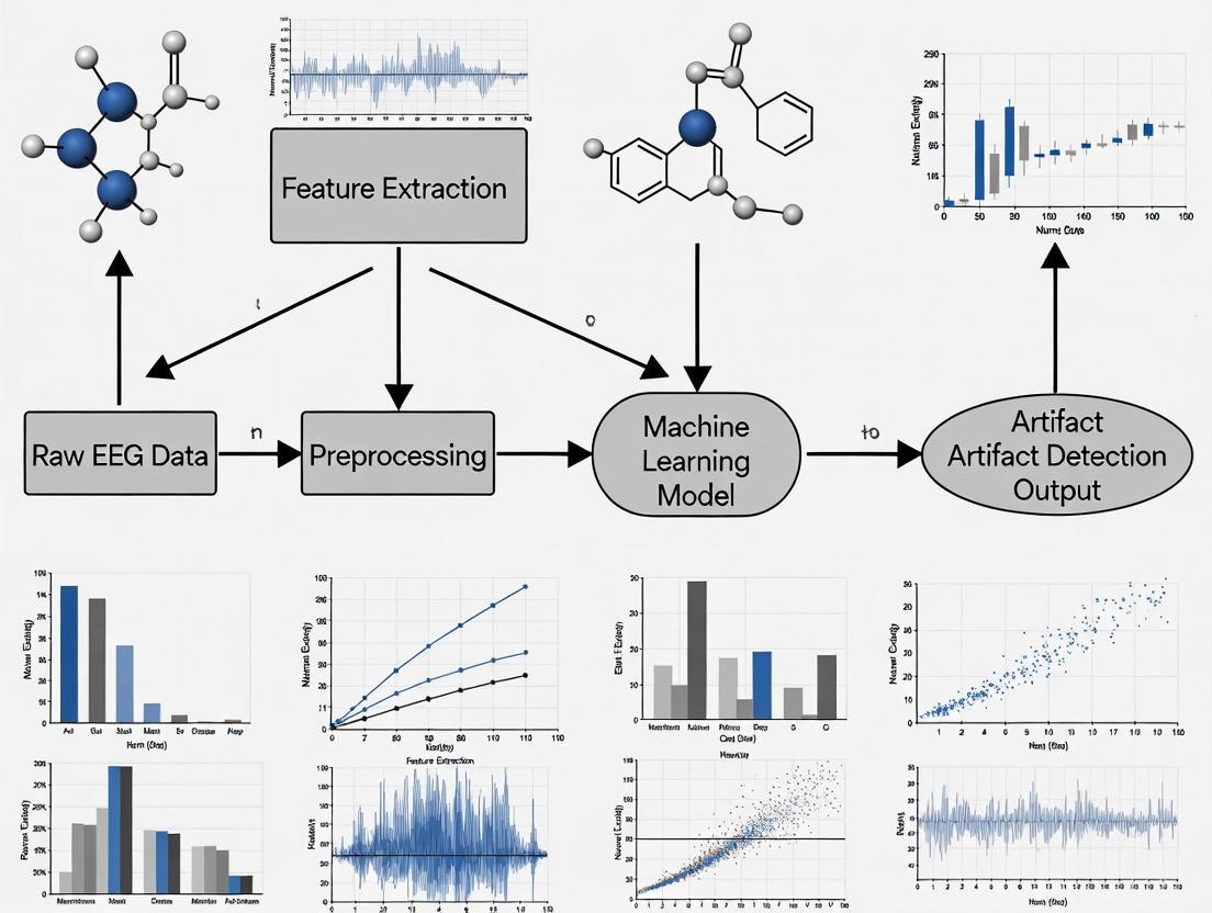
Automating artifact handling is a major focus in modern EEG research, aiming to overcome the time-consuming and subjective nature of manual review [3] [6]. The following workflow illustrates a generalized pipeline for a machine learning-based approach to this problem.
Experimental Protocol: Unsupervised Detection with LSTEEG Autoencoder This protocol is based on the methodology described by Aquilué-Llorens & Soria-Frisch [3].
- Data Preparation: Obtain a dataset of clean, pre-processed EEG epochs (e.g., from the LEMON dataset). Partition the data into training (60%), validation (20%), and test (20%) sets.
- Model Training: Train an LSTM-based autoencoder (LSTEEG) using only the clean training data. The objective is to minimize the Mean Squared Error (MSE) between the input epoch and the reconstructed output.
- Anomaly Detection: Forward new, unlabeled EEG epochs through the trained network. Calculate the reconstruction MSE.
- Classification: Epochs with low MSE are classified as "clean" (similar to training data), while epochs with high MSE are classified as "contaminated" or artifactual (anomalies). The MSE value serves as the classification metric, and performance can be evaluated using the Area Under the ROC Curve (AUC) [3].
Experimental Protocol: Supervised Correction with AnEEG (LSTM-GAN) This protocol is based on the methodology described in Scientific Reports [4].
- Data Preparation: Create a paired dataset where each input is a noisy/artifact-contaminated EEG epoch, and the corresponding target is a clean, ground-truth version of the same epoch. Ground truth can be established using advanced artifact removal techniques.
- Model Architecture: Implement a Generative Adversarial Network (GAN) where:
- The Generator is an LSTM-based network that takes the noisy EEG as input and generates a "cleaned" signal.
- The Discriminator is a Convolutional Neural Network (CNN) that tries to distinguish between the generator's output and the true clean signal.
- Adversarial Training: Train the model in a two-step iterative process. The generator learns to produce cleaned signals that are realistic enough to "fool" the discriminator, while the discriminator becomes better at identifying real vs. generated clean signals. This competition drives the generator to produce high-quality, artifact-free EEG.
- Evaluation: Use quantitative metrics like Normalized Mean Square Error (NMSE), Root Mean Square Error (RMSE), Correlation Coefficient (CC), and Signal-to-Noise Ratio (SNR) to validate the quality of the corrected signal against the ground truth [4].
The Scientist's Toolkit
Table: Key Computational Tools for Automated EEG Artifact Processing
| Tool / Reagent | Function / Application in Research |
|---|---|
| LSTM-based Autoencoder (e.g., LSTEEG) [3] | An unsupervised deep learning model that learns to compress and reconstruct clean EEG. It is leveraged for artifact detection by calculating the reconstruction error, where high error indicates an anomaly/artifact. |
| Generative Adversarial Network (GAN) [4] | A deep learning framework for artifact removal. It pits a generator (which cleans the signal) against a discriminator, leading to the synthesis of high-quality, artifact-corrected EEG data. |
| Independent Component Analysis (ICA) [3] [1] | A classical blind source separation technique used to decompose multi-channel EEG into independent components. Researchers can then manually or automatically (e.g., with ICLabel) identify and remove components correlated with artifacts. |
| Random Forest Classifier [6] | A traditional machine learning model effective for automated detection of artifacts, especially in specific contexts like single-channel, short-epoch neonatal EEG. |
| LEMON & EEGDenoiseNet Datasets [3] [4] | Publicly available benchmark EEG datasets that are essential for training, validating, and benchmarking the performance of new artifact detection and removal algorithms. |
Troubleshooting Guide: Addressing Common EEG Issues
Issue: Persistent noise or flat lines across all channels.
- Step 1: Check the basic electrode/cap connections. Ensure all components are plugged in correctly. Re-apply and check the impedance of the ground (GND) and reference (REF) electrodes, as a faulty reference can affect all channels [7] [1].
- Step 2: Restart the recording software and the amplifier unit. This can resolve temporary software glitches [7].
- Step 3: If possible, swap out the headbox and cables to rule out a hardware-level failure [7].
- Step 4: Check for external sources of electrical interference, such as unshielded power cables or electronic devices near the participant [1].
Issue: High-frequency noise on a single channel.
- Step 1: Identify the specific channel displaying the noise.
- Step 2: Inspect the corresponding electrode. Re-apply the electrode by cleaning the site and adding fresh conductive gel to ensure good skin contact and low impedance [7].
- Step 3: Check the specific cable and connector for that channel for any damage or looseness [1].
- Step 4: If the problem persists, try replacing the electrode entirely to rule out a "dead" or faulty sensor [7].
Troubleshooting Guides
Guide 1: Diagnosing Source Misclassification in Automated Artifact Detection
Problem: Your automated pipeline misclassifies high-entropy neural signals as artifacts, incorrectly rejecting valuable data.
Explanation: In the context of disorders of consciousness, high-entropy brain states are a hallmark of conscious awareness but can share temporal or spectral properties with muscle artifacts. Automated systems may mistakenly flag these valuable neural patterns as noise [8].
Solution:
- Step 1 - Verify with Ground Truth: Check if the epochs flagged as artifacts contain known neural markers. For example, confirm the presence of event-related potentials (ERPs) like P300 or N400 in the rejected trials using a separate clean dataset [9].
- Step 2 - Implement Spatial Analysis: Analyze the topographic distribution of the signal. Neural signals typically follow known spatial patterns (e.g., activity over parietal regions for certain cognitive tasks), while artifacts like muscle noise often have a more focal, frontal, or temporal distribution [8] [1].
- Step 3 - Adjust Algorithm Thresholds: If using an anomaly detection autoencoder like LSTEEG, recalibrate the threshold for the reconstruction error. Retrain or fine-tune the model on a dataset that includes high-entropy brain states to improve its discrimination capability [3].
Guide 2: Addressing Incomplete Artifact Removal in Deep Learning Models
Problem: After processing with a deep learning denoising model, residual artifacts remain in the EEG signal, potentially leading to confounds in decoding analyses.
Explanation: Deep learning models, such as the AnEEG network or LSTEEG autoencoder, are trained to reconstruct clean signals. However, with complex or high-amplitude artifacts (e.g., from motion or transcranial electrical stimulation), the model may only partially remove the noise, leaving remnants that can still skew downstream analysis [4] [3] [10].
Solution:
- Step 1 - Quality Metric Check: Calculate post-correction quality metrics like Signal-to-Artifact Ratio (SAR) and Correlation Coefficient (CC) against a ground truth. Low values indicate incomplete removal [4].
- Step 2 - Hybrid Approach: For severe artifacts, combine deep learning correction with a subsequent artifact rejection step. Models may struggle with large artifacts that completely mask brain activity; rejecting these epochs entirely preserves the integrity of the remaining data [3].
- Step 3 - Model Selection/Retraining: Benchmark different models for your specific artifact type. For instance, a multi-modular State Space Model (SSM) may outperform a convolutional network for removing artifacts from transcranial random noise stimulation (tRNS) [10]. Retrain your model on data that better represents the challenging artifacts in your experiments.
Frequently Asked Questions (FAQs)
Q1: We are using a low-density, wearable EEG system for a drug development study. Why do standard artifact removal techniques like ICA perform poorly, and what are better options?
A: Independent Component Analysis (ICA) requires a high number of channels and stable scalp coverage to effectively separate neural sources from artifacts reliably. Wearable EEG systems often have a low number of channels (typically below 16) and use dry electrodes, which reduces spatial resolution and increases signal instability, thus impairing ICA's effectiveness [11] [12]. Better options include:
- Artifact Subspace Reconstruction (ASR): An adaptive method that is widely applied for ocular, movement, and instrumental artifacts in wearable EEG [11].
- Deep Learning Models: Models like LSTM-based autoencoders (e.g., LSTEEG) or GANs (e.g., AnEEG) are emerging as powerful tools. They can learn complex, non-linear artifact representations and are particularly promising for muscular and motion artifacts in real-time settings [11] [4] [3].
Q2: Our multivariate pattern analysis (MVPA) shows good decoding accuracy, but we are concerned that residual artifacts might be creating false confounds. How can we verify this?
A: Your concern is valid, as artifacts can artificially inflate decoding accuracy. A recent study systematically evaluated this issue. The findings suggest that while a combination of artifact correction and rejection may not always significantly enhance decoding performance, artifact correction (e.g., using ICA for ocular artifacts) prior to analysis is still strongly recommended to minimize the risk of artifact-related confounds [9]. To verify your results:
- Control Analysis: Run your decoding algorithm on the artifact-free intervals only and compare the performance with the results from the full dataset. A significant drop in accuracy when using only clean data may indicate that artifacts were driving your initial results.
- Inspect Topographies: Examine the weight maps of your decoder. If the most influential features originate from channels known for artifact contamination (e.g., frontal sites for eye blinks), it suggests a potential confound [9].
Q3: For our automated pipeline, what is the most effective way to classify different types of artifacts (e.g., ocular vs. muscular) using machine learning?
A: Classifying specific artifact categories is a critical step for applying tailored removal strategies. The most effective approaches combine component analysis with deep learning:
- ICA with a Classifier: First, use ICA to decompose the EEG signal into independent components. Then, instead of manual inspection, use a trained classifier (e.g., a Convolutional Neural Network) to automatically label these components based on their topographic maps and power spectra. This method has achieved high accuracy (>91%) in classifying muscle, eye blink, and horizontal eye movement artifacts [13].
- End-to-End Deep Learning: Newer models like DSCnet are designed for multi-angle feature learning directly from EEG signals, which can capture spatiotemporal patterns characteristic of different artifacts without the need for a separate decomposition step [14].
Table 1: Performance Metrics of Selected Deep Learning Models for EEG Artifact Removal
| Model Name | Model Architecture | Key Metric | Performance Value | Primary Artifact Targeted | Reference Dataset |
|---|---|---|---|---|---|
| AnEEG | LSTM-based GAN | Correlation Coefficient (CC) | Higher than wavelet techniques | Muscle, Ocular, Environmental | [4] |
| DSCnet | Depthwise Separable CNN + DAFM | Classification Accuracy | 85.11% (Drug), 84.56% (Alcohol) | N/A (Addiction Detection) | Collected dataset, UCI [14] |
| ICA + ANN | ICA + Artificial Neural Network | Classification Accuracy | 91.01% ± 5.12% | Ocular (98.29%), EMG | 841 Healthy Subjects [13] |
| LSTEEG | LSTM-based Autoencoder | Area Under Curve (AUC) | Competitive performance shown | General Artifacts (Detection) | LEMON Dataset [3] |
| M4 Network | State Space Model (SSM) | Root Relative Mean Squared Error (RRMSE) | Best for tACS & tRNS | tES Artifacts | Synthetic tES Dataset [10] |
Table 2: Characteristics and Impacts of Common EEG Artifacts on Data Integrity
| Artifact Type | Origin | Temporal Signature | Spectral Signature | Primary Impact on Neural Signals & Risk of Skewed Results |
|---|---|---|---|---|
| Ocular (EOG) | Eye movements/blinks | Sharp, high-amplitude deflections (Frontal) | Dominates Delta/Theta bands | Masks cognitive low-frequency rhythms; can be misclassified as neural activity [1]. |
| Muscle (EMG) | Muscle contractions | High-frequency noise | Broadband, dominates Beta/Gamma | Obscures high-frequency neural oscillations related to cognition and motor activity [11] [1]. |
| Cardiac (ECG) | Heartbeat | Rhythmic waveforms | Overlaps multiple bands | Can create periodic confounds; challenging to detect without reference [1]. |
| Electrode Pop | Poor electrode contact | Abrupt, high-amplitude transients | Broadband, non-stationary | Can be misinterpreted as epileptiform spikes or other pathological neural events [1]. |
| Motion | Head/Body movement | Large, non-linear noise bursts | Varies; can mimic rhythms | Introduces non-linear drifts and noise, severely challenging signal interpretation in mobile EEG [11] [1]. |
Experimental Protocols
Protocol 1: Benchmarking Deep Learning Models for tES Artifact Removal
Objective: To evaluate and compare the performance of multiple machine learning models in removing artifacts induced by different Transcranial Electrical Stimulation (tES) modalities from simultaneous EEG recordings.
Methodology:
- Dataset Creation: A semi-synthetic dataset is created by adding clean EEG recordings with synthetically generated tES artifacts (for tDCS, tACS, and tRNS). This provides a known ground truth for rigorous evaluation [10].
- Model Training: A suite of eleven models is trained, including traditional methods and advanced deep learning architectures like Complex CNN and a multi-modular State Space Model (M4) [10].
- Performance Evaluation: Models are evaluated using three metrics calculated between the denoised output and the ground truth clean EEG:
- Root Relative Mean Squared Error (RRMSE) in temporal and spectral domains.
- Correlation Coefficient (CC) [10].
Key Workflow Diagram:
Protocol 2: Unsupervised Anomaly Detection for EEG Artifacts Using an Autoencoder
Objective: To detect artifacts in EEG signals without requiring labeled data, by treating artifacts as anomalies.
Methodology:
- Data Preparation: A dataset of clean, pre-processed EEG epochs is used (e.g., from the LEMON dataset). This data is split 60/20/20 for training, validation, and testing [3].
- Unsupervised Training: An autoencoder (e.g., LSTEEG) is trained solely on the clean EEG data. The network learns to compress and reconstruct normal brain activity by minimizing the Mean Squared Error (MSE) between its input and output [3].
- Anomaly Detection: During inference, new EEG epochs (potentially containing artifacts) are fed into the autoencoder. The reconstruction MSE is calculated for each epoch.
- A low MSE indicates the epoch is similar to the training data (i.e., clean).
- A high MSE indicates the epoch is an anomaly (i.e., contains artifacts) [3].
- Validation: The Area Under the Receiver Operating Characteristic Curve (AUC) is used to determine the predictive ability of the reconstruction MSE for classifying noisy vs. clean epochs [3].
Key Workflow Diagram:
The Scientist's Toolkit: Research Reagent Solutions
Table 3: Essential Resources for Automated EEG Artifact Detection Research
| Resource Name / Type | Function in Research | Specific Example / Note |
|---|---|---|
| Public EEG Datasets | Provides standardized data for training and benchmarking machine learning models. | EEGDenoiseNet [3]; LEMON Dataset [3]; UCI Alcohol Addiction Dataset [14]; PhysioNet Motor/Imagery Dataset [4]. |
| Blind Source Separation (BSS) | A foundational technique for decomposing EEG signals into constituent sources before classification. | Independent Component Analysis (ICA) is the most common method, used to generate components for subsequent automated classification [13] [1]. |
| Deep Learning Frameworks | Enables the development and training of complex models for end-to-end artifact detection and removal. | Used for architectures like GANs (AnEEG [4]), LSTM Autoencoders (LSTEEG [3]), CNNs, and State Space Models (M4 [10]). |
| Semi-Synthetic Data Generators | Allows for controlled evaluation by mixing clean EEG with known artifacts, providing a perfect ground truth. | Crucial for benchmarking, especially for artifacts like those from tES, where a clean reference is otherwise unavailable [10]. |
| Automated Classification Tools | Reduces or eliminates the need for manual inspection of components or signals, enabling high-throughput analysis. | ICLabel (a CNN for ICA component labeling [3]); Custom ANN classifiers for ICA components [13]. |
Electroencephalography (EEG) is a crucial tool in neuroscience and clinical diagnostics, but its signals are frequently contaminated by artifacts from biological sources (eye movements, muscle activity, cardiac rhythms) and environmental sources (powerline interference, electrode movement) [4]. These artifacts obscure neural information and can lead to misinterpretation in both research and clinical settings. For decades, traditional methods like Blind Source Separation (BSS) and rule-based thresholding have formed the cornerstone of EEG artifact management. However, within the context of advancing automatic artifact detection using machine learning, understanding the specific limitations of these traditional approaches becomes paramount. This technical support guide examines these limitations through experimental evidence and provides troubleshooting guidance for researchers navigating these methodological challenges.
Understanding Blind Source Separation (BSS) and Its Limitations
Blind Source Separation, particularly Independent Component Analysis (ICA), has been a prominent processing tool in EEG research for separating intracranial dipolar sources from scalp recordings without relying on head modeling [15]. BSS operates on the superposition principle, where scalp potentials are represented as a linear, instantaneous mixture of underlying neural sources [16].
Core Technical Limitation: Sensitivity to Mixing Matrix Distortions
A fundamental assumption of BSS is that the mixing matrix remains invariant—meaning sources, electrodes, and head geometry do not change during recording. In practice, this assumption is frequently violated.
Troubleshooting FAQ: BSS Component Proliferation
- Q: My BSS analysis is identifying more components than expected, with many having similar properties. What is causing this, and how can I troubleshoot it?
- A: This is a common problem linked to violations of the mixing matrix invariance assumption. Even slight electrode movement or inter-individual anatomo-functional variability in group analyses creates non-Gaussian features that impair Higher-Order Statistics (HOS) algorithms [16]. To troubleshoot:
- Inspect Data Stationarity: Check for segments where electrode impedance may have changed or where head movement occurred.
- Compare Algorithms: Test Second-Order Statistics (SOS) algorithms like SOBI or AJDC, which are more robust to these distortions [16].
- For Group ICA: Avoid using a single mixing matrix for all subjects. Consider alternative approaches that account for inter-subject variability.
Experimental Protocol: Testing BSS Robustness
- Objective: To evaluate the sensitivity of different BSS algorithms to controlled distortions in the mixing matrix.
- Method (as simulated in [16]):
- Generate Synthetic Data: Create artificial EEG data from known dipolar sources with a stable mixing matrix.
- Introduce Distortion: Simulate a sudden electrode displacement by abruptly altering the mixing coefficients for a subset of channels.
- Apply BSS Algorithms: Process the distorted data with multiple HOS-based (e.g., FASTICA, INFOMAX) and SOS-based (e.g., SOBI, AJDC) algorithms.
- Evaluate Performance: Measure the quality of recovered signals and the accuracy of source localization for each algorithm.
- Key Finding: HOS-based methods are substantially more impaired by mixing matrix distortions, leading to the identification of spurious components and reduced localization efficiency [16].
Table 1: Comparison of BSS Algorithm Performance Under Mixing Matrix Distortions
| Algorithm Type | Example Algorithms | Robustness to Mixing Matrix Distortion | Impact on Source Recovery |
|---|---|---|---|
| Higher-Order Statistics (HOS) | FASTICA, INFOMAX, Ext-INFOMAX | Low | Substantial impairment; creates non-Gaussian features, leading to more components than actual sources [16]. |
| Second-Order Statistics (SOS) | SOBI, UW-SOBI, AJDC | High | Significantly less sensitive; better recovery of signal quality and localization accuracy [16]. |
| Hybrid Algorithms | JADE, COMBI | Moderate | Variable performance, often intermediate between SOS and HOS [16]. |
Workflow Diagram: BSS Analysis and Problem Identification
The following diagram illustrates a standard BSS workflow and pinpoints where the critical limitation of mixing matrix invariance can manifest.
The Thresholding Problem in Rule-Based Methods
Rule-based methods often rely on graph theoretical analyses of functional connectivity, which require thresholding to eliminate spurious connections. The choice of this threshold is arbitrary and represents a significant source of variability.
Core Technical Limitation: Arbitrary Threshold Selection
The arbitrary choice of a proportional threshold dramatically influences the global metrics of a functional connectivity network.
Troubleshooting FAQ: Inconsistent Graph Metrics
- Q: The global connectivity measures from my EEG functional connectivity analysis change drastically with different proportional thresholds. How can I ensure the stability and validity of my results?
- A: This is known as the "thresholding problem" [17]. To improve robustness:
- Avoid Single Thresholds: Do not base conclusions on a single, arbitrarily chosen threshold.
- Threshold-Free or Multi-Threshold Analysis: Explore threshold-free measures or report results across a range of plausible thresholds to demonstrate the stability of your findings.
- Improve Reasoning: Document and justify the chosen thresholding method in your analysis protocol. The field is moving towards improved reasoning behind analytic choices and the adoption of different approaches [17].
Experimental Protocol: Quantifying Thresholding Variability
- Objective: To demonstrate the effect of proportional thresholding on graph network parameters.
- Method (as conducted in [17]):
- Data Acquisition: Collect resting-state EEG from participants (e.g., 146 recordings).
- Compute Functional Connectivity: Calculate connectivity matrices using multiple synchronization measures (e.g., wPLI, ImCoh, Coherence).
- Apply Thresholding: Apply a series of proportional thresholds (e.g., from 5% to 30% strongest connections retained) to each matrix.
- Calculate Graph Metrics: For each thresholded matrix, compute global graph metrics such as clustering coefficient, path length, and small-worldness.
- Analyze Variability: Plot the graph metrics as a function of the applied threshold.
- Key Finding: Graph network parameters show significant changes as a function of the chosen threshold, which can directly influence the outcome and conclusions of a study [17].
Table 2: Impact of Proportional Thresholding on Global Graph Metrics (Sample Observations from [17])
| Proportional Threshold (% of strongest connections) | Effect on Clustering Coefficient | Effect on Characteristic Path Length | Risk of Conclusion Bias |
|---|---|---|---|
| Low (e.g., 5-10%) | May be artificially high due to inclusion of spurious weak connections. | May be artificially low. | High: Network may appear erroneously integrated. |
| Medium (e.g., 15-20%) | Potentially reflects true network structure, but "true" value is unknown. | Potentially reflects true network structure. | Medium: Highly dependent on sample and measure. |
| High (e.g., 25-30%) | May be artificially low due to oversparsification of the network. | May be artificially high. | High: Network may appear erroneously segregated. |
The Scientist's Toolkit: Key Research Reagents & Materials
Table 3: Essential Tools for EEG Artifact Research
| Item / resource | Function / purpose | Example / note |
|---|---|---|
| EEGLAB | An open-source MATLAB toolbox for processing single-trial EEG dynamics, including ICA [18]. | Provides a framework for BSS analysis, visualization, and plugin management (e.g., FIRFILT plugin). |
| TUH EEG Artifact Corpus | A public dataset of clinical EEG with expert-annotated artifacts [19]. | Used for training and validating automated artifact detection models; contains 158k+ annotations. |
| Standardized Montages | A predefined set of electrode pairs for bipolar derivation. | Reduces common-mode noise; essential for standardizing inputs to deep learning models [19]. |
| SOS BSS Algorithms (e.g., SOBI, AJDC) | For source separation when data violates the mixing matrix invariance assumption [16]. | More robust than HOS algorithms to electrode movement and group-level analysis. |
| Deep Learning Frameworks (e.g., TensorFlow, PyTorch) | For building and training specialized artifact detection models. | Enables development of CNNs and other architectures tailored to specific artifact classes [19]. |
Comparative Analysis: Traditional vs. Modern Approaches
The limitations of traditional methods have catalyzed the development of novel approaches, particularly deep learning models.
Troubleshooting FAQ: Choosing an Artifact Handling Strategy
- Q: With the rise of deep learning, should I abandon traditional methods like BSS and rule-based thresholding for artifact management?
- A: Not necessarily. The choice of method should be guided by your specific research context:
- For Well-Defined, Stationary Data: Traditional BSS can still be effective and offers interpretability.
- For Clinical or Noisy Data: Consider SOS-based BSS for its robustness or explore modern deep learning models.
- For Automated, High-Throughput Processing: Specialized deep learning models are superior. Research shows that artifact-specific Convolutional Neural Networks (CNNs) significantly outperform rule-based methods, with F1-score improvements from +11.2% to +44.9% [19]. These models can be optimized for specific artifacts (e.g., 1s windows for non-physiological, 20s for eye movements) [19].
- For Functional Connectivity: Move beyond single-threshold analyses and employ multi-threshold or threshold-free techniques to ensure the robustness of your findings [17].
Table 4: Comparison of Artifact Handling Methodologies
| Methodology | Key Principle | Primary Limitations | Best-Suited Context |
|---|---|---|---|
| BSS (HOS - ICA) | Separates sources by maximizing statistical independence using higher-order statistics [15]. | Highly sensitive to mixing matrix distortions; can create spurious components [16]. | Single-subject research data with minimal head/electrode movement. |
| BSS (SOS - SOBI) | Separates sources using second-order statistics (temporal correlations) [16]. | More robust to mixing matrix non-stationarity but may have other computational limitations [16]. | Data with suspected instability (e.g., group studies, long recordings). |
| Rule-Based Thresholding | Applies fixed rules or thresholds to exclude artifactual data segments or connections. | Arbitrary threshold selection dramatically alters graph network parameters [17]. | Initial, exploratory data screening; requires careful validation. |
| Deep Learning (e.g., CNN) | Learns artifact features directly from large, labeled datasets through hierarchical feature detection [19]. | Requires large annotated datasets; "black box" nature can reduce interpretability [19]. | High-accuracy, automated detection of specific artifact classes in large datasets. |
| Hybrid Expert Schemes | Combines signal processing (e.g., energy screening) with rule-based expert knowledge [20]. | Requires careful design to encode expert knowledge effectively; may be complex to implement. | Tasks requiring precise localization and duration of specific micro-events (e.g., K-complex detection in sleep EEG) [20]. |
The limitations of traditional BSS and rule-based thresholding are not merely theoretical but have demonstrable, quantifiable impacts on EEG data analysis, as evidenced by the experimental protocols and data summarized here. The fundamental constraints of mixing matrix invariance and arbitrary threshold selection can introduce bias, variability, and spurious findings. The field is now moving toward a new paradigm characterized by more robust second-order statistics, sophisticated hybrid models that integrate expert knowledge, and specialized deep learning systems. These advanced methods offer a path toward fully automated, accurate, and reliable artifact handling, which is essential for the progression of robust machine learning applications in EEG research.
Frequently Asked Questions (FAQs)
FAQ 1: What are the most common types of EEG artifacts I should account for in my automated detection model?
EEG artifacts can be broadly categorized as physiological (from the body) or technical (from equipment or environment). The table below summarizes the common artifacts and recommended detection methods.
| Artifact Type | Origin | Key Characteristics | Recommended ML Detection Methods |
|---|---|---|---|
| Eye Blinks & Movements [21] | Physiological (Eyes) | High-amplitude, slow deflections; frontally prominent. [21] | ICA, Template matching on EOG channels. [22] [23] |
| Muscle Artifacts (EMG) [21] | Physiological (Muscles) | High-frequency, broadband activity; most prominent above 20 Hz. [21] | ICA, Time-frequency analysis, Band-power features. [21] |
| Heartbeat Artifacts (ECG) [21] | Physiological (Heart) | Rhythmic, spike-shaped pattern; can be confounded with epileptiform activity. [21] | ICA, SSP with ECG channel correlation. [22] [23] |
| Line Noise [21] | Technical (Environment) | Sharp peak at 50/60 Hz and its harmonics. [21] | Notch filtering, Spectral analysis. [21] |
| Electrode "Pops" [21] | Technical (Electrode) | Sudden, large-amplitude, instantaneous deflection. [21] | Amplitude-thresholding, Statistical outlier detection. [21] |
| Sweat/Skin Potentials [21] | Physiological (Skin) | Very slow drifts and fluctuations. [21] | High-pass filtering, Drift-correction algorithms. [21] |
FAQ 2: My deep learning model for seizure detection is overfitting on my limited EEG dataset. What strategies can I use?
Overfitting is a common challenge, especially with small-sample EEG datasets [24]. You can employ several strategies:
- Data Augmentation: Use techniques like sliding windows with overlaps to artificially expand your dataset [24]. For a 23.6-second EEG file, using a 1-second sliding window can generate multiple samples, increasing the effective dataset size for training.
- Simplified Model Architectures: Instead of large, complex networks, use streamlined models designed for small data. For example, one study proposed a "micro-capsule network" that maintains high accuracy with reduced computational complexity and lower risk of overfitting [24].
- Transfer Learning: Leverage pre-trained models or general-purpose features learned from larger datasets and adapt them to your specific task with a smaller amount of patient-specific data [25].
FAQ 3: How can I create a model that works well across different subjects and tasks (cross-subject/cross-task)?
This is a core challenge in building generalizable EEG foundation models. The 2025 EEG Foundation Challenge highlights two key approaches [26]:
- Cross-Task Transfer Learning: Develop models using unsupervised or self-supervised pre-training on data from various cognitive tasks (e.g., resting state, movie watching). The model learns general latent EEG representations, which are then fine-tuned for a specific supervised task like predicting behavioral performance [26].
- Subject-Invariant Representations: Create robust models that explicitly learn to ignore subject-specific morphological and physiological differences. This often involves training on data from a large number of participants (e.g., 3,000+) across multiple paradigms to force the model to find common, task-related features [26].
FAQ 4: What are the trade-offs between traditional machine learning and deep learning for artifact detection?
The choice between traditional Machine Learning (ML) and Deep Learning (DL) depends on your data and resources.
| Feature | Traditional Machine Learning | Deep Learning |
|---|---|---|
| Data Dependency | Performs better with smaller datasets [24]. | Requires large datasets to avoid overfitting [24]. |
| Feature Engineering | Relies on manual feature extraction (e.g., statistical moments, entropy, bandpower) [27] [25]. | Automatic feature learning from raw or preprocessed data [27] [25]. |
| Computational Load | Generally less computationally intensive. | Can be very computationally intensive, requiring high hardware resources [24]. |
| Interpretability | Often more interpretable (e.g., knowing which feature is important). | Acts as a "black box," making it harder to understand decisions [24]. |
| Best Use Case | Well-defined artifacts with known characteristics on small-to-medium datasets. | Complex artifact patterns or when manual feature extraction is impractical on large datasets. |
Troubleshooting Guides
Issue 1: Poor performance of my artifact detection algorithm due to overlapping signal and artifact frequencies.
Problem: Some artifacts, like muscle activity, have a broad frequency spectrum that overlaps with the EEG signal of interest (e.g., beta and gamma bands), making simple frequency filtering ineffective [21].
Solution: Employ component-based methods that leverage spatial information.
- Use Independent Component Analysis (ICA): ICA can separate EEG recordings into statistically independent components. Artifacts like blinks, eye movements, and heartbeats often map to distinct components that can be identified and removed [21].
- Identify Artifact Components: Correlate components with reference EOG and ECG channels to automatically identify those corresponding to artifacts. Components with topographies focused on the eyes (for blinks) or temples (for saccades) and time courses that match the artifact can be selected for rejection [22] [23].
- Reconstruct Signal: Remove the identified artifact components and reconstruct the "cleaned" EEG signal.
The following workflow outlines this component-based approach to artifact removal:
Issue 2: My model fails to generalize and performs poorly on new, unseen subject data.
Problem: High inter-subject variability in EEG signals causes models trained on one group of subjects to perform poorly on others [25].
Solution: Implement a Ensemble of Deep Transfer Learning (EDTL) strategy [25].
- Leverage Pre-trained Models: Start with general-purpose models pre-trained on large-scale datasets (e.g., ResNet, EfficientNet) to capture universal features.
- Incorporate Domain-Specific Models: Combine the pre-trained models with a custom 2D Convolutional Neural Network (2DCNN) designed for your specific EEG data characteristics.
- Create Patient-Specific Features: Use techniques like Short-Time Fourier Transform (STFT) to convert EEG signals into spectrograms, which can better capture time-frequency patterns for individual patients.
- Ensemble the Models: Combine the predictions of the pre-trained models and the custom 2DCNN. This ensemble approach improves robustness against noise and enhances adaptability to new subjects [25].
The workflow below illustrates the key steps in creating a generalizable, subject-invariant model using transfer learning and ensemble methods:
The Scientist's Toolkit: Essential Research Reagents & Materials
The following table lists key computational tools and materials used in modern ML-based EEG artifact detection research.
| Item Name | Function / Application |
|---|---|
| HBN-EEG Dataset [26] | A large-scale public dataset with over 3,000 participants across six tasks, ideal for training and benchmarking generalizable foundation models. [26] |
| CHB-MIT Scalp EEG Database [27] [25] | A standard public dataset for epileptic seizure detection, widely used to validate and compare the performance of new algorithms. [27] [25] |
| Bonn EEG Dataset [24] | A public dataset containing EEG recordings categorized into epilepsy-specific stages, often used for small-sample method development. [24] |
| Independent Component Analysis (ICA) [21] | A computational method used to separate mixed EEG signals into independent sources, crucial for isolating and removing artifact components. [21] |
| Short-Time Fourier Transform (STFT) [25] | A signal processing technique that converts 1D EEG time-series into 2D spectrograms (time-frequency representations), used as input for image-based deep learning models like CNNs. [25] |
| Micro-Capsule Network [24] | A streamlined deep learning architecture designed to effectively learn from small-sample EEG datasets by preserving spatial hierarchical relationships in the data. [24] |
| Python MNE Library [23] | An open-source Python package for exploring, visualizing, and analyzing human neurophysiological data, providing standard preprocessing and artifact detection tools. [23] |
Frequently Asked Questions (FAQs)
Q1: What are the most common artifacts that can compromise EEG data in clinical trials? EEG artifacts are any recorded signals not originating from neural activity. They are broadly categorized as follows [1]:
- Physiological Artifacts: Originate from the participant's body.
- Ocular Artifacts: From eye blinks and movements (high-amplitude, low-frequency), affecting frontal electrodes.
- Muscle Artifacts (EMG): From jaw, face, or neck muscle contractions (broadband, high-frequency noise).
- Cardiac Artifacts (ECG): Rhythmic waveforms from heartbeats.
- Perspiration/Respiration: Cause slow baseline drifts and impedance changes.
- Non-Physiological Artifacts: Originate from external sources.
- Electrode Pop: Sudden, high-amplitude transients from poor electrode-skin contact.
- Cable Movement: Creates variable noise from cable displacement.
- AC Power Line Interference: A sharp 50/60 Hz noise from electrical environments.
Q2: Why is automated artifact detection crucial for modern drug development trials? Manual artifact review is time-consuming, labor-intensive, and subjective, which is not feasible for large-scale, multi-site clinical trials. Automated methods based on machine learning (ML) and deep learning (DL) ensure standardized, reproducible, and scalable data preprocessing. This enhances the reliability of EEG biomarkers as endpoints by reducing human error and bias, which is critical for regulatory acceptance [28].
Q3: My trial uses wearable EEG devices. Are there special considerations for artifact handling? Yes. Wearable EEG systems, which often use dry electrodes and have a low number of channels, present specific challenges [11]:
- Increased Artifact Proneness: Dry electrodes and subject mobility introduce more motion artifacts and signal instability.
- Limited Spatial Resolution: A reduced number of channels (often below 16) impairs the effectiveness of traditional source separation methods like Independent Component Analysis (ICA).
- Emerging Solutions: Techniques like Artifact Subspace Reconstruction (ASR) and deep learning models are being validated for wearable EEG. The use of auxiliary sensors (e.g., IMUs) is promising but currently underutilized [11].
Q4: How do I choose between a traditional algorithm and a deep learning model for my study? The choice depends on your data, resources, and goals. The table below summarizes key considerations based on published research [19] [29] [28].
| Method | Best For | Key Advantages | Limitations |
|---|---|---|---|
| Independent Component Analysis (ICA) | Studies with sufficient channels (e.g., >16); isolating ocular and muscular artifacts [11] [1]. | Well-established, interpretable, does not require labeled data. | Requires expert intervention for component rejection, less effective for low-density EEG [11]. |
| Machine Learning (e.g., Random Forest) | Small to medium-sized datasets; scenarios requiring high accuracy with limited training data [28]. | High performance with smaller datasets, fast training and inference. | Requires manual feature engineering in many implementations. |
| Deep Learning (CNN, LSTM, Autoencoders) | Large, labeled datasets; complex artifacts (muscle, motion); end-to-end learning [19] [29] [30]. | Automatic feature extraction, state-of-the-art accuracy, handles complex patterns. | Requires large amounts of training data; acts as a "black box"; computationally intensive [28]. |
Q5: What are the key performance metrics for evaluating an artifact detection algorithm? The choice of metrics depends on whether the task is detection (classifying an epoch as artifact/noise) or removal (reconstructing a clean signal). Commonly used metrics include [11]:
- For Detection:
- Accuracy: Overall correctness.
- Selectivity (True Negative Rate): Ability to identify clean segments correctly.
- For Removal/Reconstruction:
- Signal-to-Noise Ratio (SNR): Measures noise reduction.
- Correlation Coefficient (CC): Measures waveform preservation.
- Root Mean Square Error (RMSE): Quantifies difference from a clean reference.
Troubleshooting Guides
Guide 1: Resolving Poor Algorithm Performance on Your Dataset
Problem: Your artifact detection model is underperforming, showing low accuracy or high false positives.
Solution: Follow this systematic troubleshooting workflow.
Steps:
- Data Quality & Preprocessing Check
- Ensure consistent preprocessing (bandpass filtering, notch filtering, referencing) across all datasets [19].
- Verify that your training data is representative of the clinical trial population and conditions (e.g., same type of EEG headset, similar patient demographics).
- Audit your labels. Inconsistent or inaccurate ground truth annotations are a major source of failure. Ensure high inter-rater agreement if labeled manually [19].
Model & Training Check
- Assess model-task fit. A model trained on adult EEG may fail on infant EEG due to different artifact characteristics [28].
- Optimize hyperparameters like temporal window size. Research shows optimal windows vary by artifact: 1s for non-physiological, 5s for muscle, and 20s for eye movements [19].
- If you have a small dataset, prioritize traditional ML models like Random Forest, which can outperform deep learning in data-scarce scenarios [28].
Strategy Check
- For complex data with multiple artifact types, consider using specialized models for each artifact class instead of a single, generic model [19].
- When working with multi-channel data, ensure your model architecture (e.g., CLEnet) can leverage spatial relationships between channels, unlike models designed for single-channel input [29].
Guide 2: Implementing a Robust Artifact Handling Pipeline
Problem: You need to establish a standardized, end-to-end pipeline for artifact detection and removal in your trial's analysis plan.
Solution: Adopt a modular pipeline that can be tailored to your specific endpoint.
Steps:
- Standardized Preprocessing: Apply consistent filtering (e.g., 1-40 Hz bandpass, 50/60 Hz notch) and re-reference all data. This ensures uniformity before artifact handling [19].
- Choose a Detection Method: Select a method based on the FAQ and Table 1. For a balanced approach, a Random Forest classifier offers high accuracy and is less sensitive to dataset size [28].
- Select a Handling Strategy: This is a critical choice that depends on your trial's statistical power and endpoint.
- Epoch Rejection: Simply discard data segments flagged as artifacts. This is safe but can lead to significant data loss, which may be unacceptable in trials with limited recording time.
- Artifact Correction: Use techniques like ICA or advanced deep learning models (e.g., CLEnet, LSTEEG) to reconstruct the clean neural signal. This preserves data volume but requires rigorous validation to ensure neural signals are not distorted [29] [30].
- Validation and Reporting: Always report the percentage of data rejected or corrected in your analysis. Validate the pipeline on a held-out test set with expert annotations to ensure its performance meets the trial's quality standards.
Experimental Protocols & Benchmarking
Key Experimental Metrics from Current Literature
The following table summarizes quantitative performance data from recent studies to help you benchmark your own systems. Note that performance is highly dataset-dependent.
| Model / Approach | Artifact Type | Performance Metrics | Reference / Dataset |
|---|---|---|---|
| Deep Lightweight CNN | Eye Movements | ROC AUC: 0.975 | Temple University Hospital (TUH) EEG Corpus [19] |
| Deep Lightweight CNN | Muscle Activity | Accuracy: 93.2% | Temple University Hospital (TUH) EEG Corpus [19] |
| Deep Lightweight CNN | Non-Physiological | F1-Score: 77.4% | Temple University Hospital (TUH) EEG Corpus [19] |
| CLEnet (CNN + LSTM) | Mixed (EMG + EOG) | SNR: 11.498 dB, CC: 0.925 | EEGdenoiseNet [29] |
| Random Forest | General (Infant EEG) | Balanced Accuracy: 0.873 | BRISE Infant Dataset [28] |
| Deep Learning Model | General (Infant EEG) | Balanced Accuracy: 0.881 | BRISE Infant Dataset [28] |
| LSTEEG (LSTM Autoencoder) | General | Superior to convolutional autoencoders in detection & correction | Study-specific dataset [30] |
| Item | Function & Application | Example / Note |
|---|---|---|
| Public EEG Datasets | For training, validating, and benchmarking models. | Temple University Hospital (TUH) EEG Corpus (includes artifact labels) [19]; EEGdenoiseNet (semi-synthetic data for removal) [29]. |
| Standardized Preprocessing Tools | To apply consistent filtering, referencing, and epoching. | Toolboxes like MNE-Python, EEGLAB. Implementation should follow published protocols [19]. |
| Blind Source Separation (BSS) Tools | For traditional artifact removal methods. | Implementations of ICA (e.g., in EEGLAB) are useful for comparison and specific use cases [11] [1]. |
| Deep Learning Frameworks | For building and training state-of-the-art artifact models. | TensorFlow or PyTorch. Used to implement architectures like CNNs, LSTMs, and Autoencoders [19] [29] [30]. |
| Auxiliary Sensors | To provide additional data streams for improved artifact detection in mobile/wearable settings. | Inertial Measurement Units (IMUs) to track motion. Still underutilized but with high potential [11]. |
Machine Learning Architectures for EEG Artifact Detection: From CNNs to Hybrid Models
Frequently Asked Questions (FAQs)
Q1: What are the main advantages of using specialized, artifact-specific CNN models over a single general-purpose model?
Using multiple CNN systems, each specialized for a specific artifact class, significantly outperforms approaches that use a single model for all artifacts. Research shows that artifact-specific models allow for optimization of critical parameters, such as temporal window length, to match the unique characteristics of each artifact type. For instance, optimal window lengths were found to be 20 seconds for eye movements, 5 seconds for muscle activity, and 1 second for non-physiological artifacts [19]. This tailored approach has demonstrated F1-score improvements of +11.2% to +44.9% over traditional rule-based methods [19].
Q2: My model performs well on training data but poorly on new patient data. How can I improve its generalizability?
This is a common challenge, often stemming from the "one-size-fits-all" assumption that artifact characteristics are similar across all subjects and recording conditions [19]. To improve generalizability:
- Utilize Transfer Learning: Start with a generalized model pre-trained on a large, diverse dataset. This model can then be efficiently retrained with a limited amount of data from a new acquisition system or patient group to form a data-specific model, a process shown to be effective in iEEG studies [31].
- Employ Data Augmentation: Increase the effective size and diversity of your training dataset using techniques such as adding Gaussian white noise, using sliding windows, or employing Generative Adversarial Networks (GANs) to create synthetic EEG examples [32].
- Ensure Dataset Diversity: Train your model on datasets that feature a wide range of artifact types, recording conditions, and patient populations, such as the Temple University Hospital (TUH) EEG Corpus, which is representative of real clinical settings [19].
Q3: How do I choose the right input representation (e.g., raw signal vs. time-frequency images) for my CNN?
The choice depends on the nature of the artifacts you are targeting and the network architecture.
- 1D-CNN for Raw Waveforms: Treating the time-series as a 1D image allows the CNN to learn features directly from the raw signal without the need for manual feature extraction, making it a powerful and efficient option [31]. This approach has been successfully applied in speech recognition and biological signal processing [31].
- 2D-CNN for Time-Frequency Images: Transforming the signal into a time-frequency representation (e.g., using Fourier or Wavelet transforms) can be beneficial. CNNs excel at processing these 2D images and can leverage their strong pattern recognition capabilities to identify distinctive artifact signatures in the time-frequency plane [31].
- Spatio-Temporal Processing: If your electrode spatial information is known, you can use CNNs to process multi-channel EEG data, allowing the model to learn both the spatial and temporal characteristics of artifacts [31].
Q4: What are the alternatives if I lack a large, expertly labeled dataset for training?
A lack of labeled data is a major constraint. Consider these alternative deep-learning approaches that reduce labeling dependency:
- Autoencoders for Anomaly Detection: Train a convolutional autoencoder (CAE) exclusively on clean, artifact-free EEG data. The model learns to reconstruct normal brain signals. During inference, contaminated segments will have a high reconstruction error, which can be used as an anomaly metric to detect artifacts without needing labels for the artifacts themselves [3]. This approach has achieved high accuracy (95.5%) in detecting unseen artifacts in other biological signal domains [33].
- Leverage Pre-trained Models: Use existing, validated models like ICLabel, which is a CNN designed to classify independent components derived from ICA, to automate the initial stages of your preprocessing pipeline [3].
Troubleshooting Guides
Problem: Model Fails to Distinguish Pathological Activity from Artifacts
Issue: The CNN misclassifies epileptiform activity (e.g., interictal spikes) as artifacts, which is a critical error in clinical applications like epilepsy evaluation.
Diagnosis and Solution: This occurs because some pathological activities and artifacts share similar characteristics in the signal [31]. The model must be explicitly designed to avoid this mutual misclassification.
- Step 1: Curate Targeted Training Labels: Ensure your ground truth annotations are performed by experts who can accurately differentiate between, for example, a pathological spike and an electrode pop artifact. The training data must reflect this crucial distinction.
- Step 2: Incorporate Spatial Information: Use a multi-channel CNN architecture that can learn the spatial distribution of signals across the scalp. Genuine neural activity follows logical topographic fields of distribution, which can help the model distinguish it from artifacts [1].
- Step 3: Algorithm Design Priority: Select or design a model with this specific requirement in mind. For instance, one CNN method for iEEG was explicitly "designed to meet the condition" of avoiding misclassification between pathological high-frequency oscillations and artifacts [31].
Problem: Inconsistent Model Performance Across Different Artifact Types
Issue: The model detects certain artifacts (e.g., eye blinks) with high accuracy but performs poorly on others (e.g., muscle noise or electrode pops).
Diagnosis and Solution: A single model configuration is not optimal for the diverse temporal and spectral characteristics of different artifacts.
- Step 1: Adopt a Multi-Model Framework: Do not rely on a single CNN. Instead, deploy a system of specialized, lightweight CNNs, where each is optimized for a specific artifact class (e.g., one for eye movements, one for muscle activity, and one for non-physiological artifacts) [19].
- Step 2: Optimize Hyperparameters per Artifact: Tune the architecture and parameters for each specialized model. The most critical parameter is the input segment length, as each artifact type has a distinct optimal temporal window for detection [19].
- Step 3: Ensemble Predictions: Combine the outputs from your specialized CNNs to generate a final, comprehensive artifact profile for the EEG signal.
Workflow: Implementing an Artifact-Specific CNN Framework
Problem: High Computational Cost and Slow Training Times
Issue: Training deep CNNs on large, high-density EEG datasets is slow and computationally expensive.
Diagnosis and Solution: Complex models and large datasets naturally require significant resources. However, several strategies can mitigate this.
- Step 1: Use Lightweight Architectures: Design or select "deep lightweight" CNN architectures that maintain high accuracy with fewer parameters, making them faster to train and more suitable for deployment [19].
- Step 2: Leverage Transfer Learning: Instead of training from scratch, take a pre-trained generalized model and retrain (fine-tune) only the final layers with your specific data. This process is significantly faster and requires less data [31].
- Step 3: Utilize Hardware Acceleration: Perform training on systems with Graphical Processing Units (GPUs), which are specifically designed for the parallel computations required by CNNs and can dramatically speed up the process [31].
Experimental Protocols & Performance Data
Key Experimental Methodology for Training an Artifact-Specific CNN
The following protocol is synthesized from recent studies on artifact-specific CNNs [19]:
- Data Sourcing: Obtain EEG data from a large, publicly available corpus with expert artifact annotations, such as the Temple University Hospital (TUH) EEG Corpus.
- Preprocessing:
- Resampling: Standardize the sampling rate across all recordings (e.g., to 250 Hz).
- Filtering: Apply a bandpass filter (e.g., 1-40 Hz) and a notch filter (50/60 Hz) to remove line noise.
- Montage: Convert all recordings to a standardized bipolar montage.
- Normalization: Use a method like RobustScaler to normalize data across channels and timepoints.
- Adaptive Segmentation: Segment the continuous EEG into non-overlapping windows. Critically, use different window lengths optimized for each artifact class (e.g., 20s for eye, 5s for muscle, 1s for non-physiological).
- Model Training: Train separate CNN architectures for each artifact class. The architecture for each can be a relatively simple stack of convolutional, pooling, and fully connected layers.
- Performance Validation: Evaluate the model on a held-out test set and compare its performance (F1-score, Accuracy, ROC AUC) against standard rule-based detection methods.
Quantitative Performance of CNN Models for EEG Artifact Detection
The table below summarizes the demonstrated performance of CNN-based approaches for detecting various types of EEG artifacts.
| Artifact Type | Model Approach | Key Performance Metric | Reported Score | Context & Notes |
|---|---|---|---|---|
| General iEEG Artifacts | Convolutional Neural Network | F1-Score (Generalized Model) | 0.81 | Trained on one dataset, tested on another [31]. |
| F1-Score (Specialized Model) | 0.96 | Retrained on target dataset via transfer learning [31]. | ||
| Eye Movements | Specialized Lightweight CNN | ROC AUC | 0.975 | Optimal 20s window [19]. |
| Muscle Activity | Specialized Lightweight CNN | Accuracy | 93.2% | Optimal 5s window [19]. |
| Non-Physiological | Specialized Lightweight CNN | F1-Score | 77.4% | Optimal 1s window [19]. |
| Eye Blink Artifacts | 10-layer CNN | Classification Accuracy | 99.67% | Study on 30 subjects [32]. |
Research Reagent Solutions: Essential Materials & Tools
The table below lists key computational "reagents" and resources essential for developing artifact-specific CNNs for EEG.
| Resource Name | Type | Primary Function in Research |
|---|---|---|
| TUH EEG Artifact Corpus [19] | Dataset | Provides a large volume of expert-annotated, real-world EEG data for training and benchmarking artifact detection models. |
| ICLabel [3] | Pre-trained Model / Tool | A CNN-based tool that automates the classification of Independent Components (ICs) derived from ICA, streamlining a common preprocessing step. |
| EEGDenoiseNet [3] | Benchmark Dataset | A dataset designed specifically for training and benchmarking deep learning models for EEG denoising. |
| TensorFlow2 Object Detection API [34] | Software Library | An open-source framework that can be adapted for building and training object detection models, which can be repurposed for 1D signal detection tasks. |
| RobustScaler [19] | Preprocessing Algorithm | A data normalization technique that preserves relative amplitude relationships between EEG channels while standardizing the input for stable model training. |
Frequently Asked Questions (FAQs)
FAQ 1: Why is a single temporal window size not optimal for detecting all artifact classes? Different biological and non-biological artifacts have distinct temporal and spectral characteristics. For instance, eye movements are slow and span several seconds, while muscle artifacts are rapid and brief. Using a single window size fails to capture these unique dynamics effectively. Research has confirmed that specialized models with optimized window sizes significantly outperform generic approaches, with one study finding optimal windows of 20 seconds for eye movements, 5 seconds for muscle activity, and 1 second for non-physiological artifacts [19].
FAQ 2: How does an improperly chosen temporal window impact model performance? An incorrectly sized temporal window can lead to two main issues:
- Too short a window: May fail to capture the complete morphology of long-duration artifacts (e.g., eye rolls), missing crucial contextual information.
- Too long a window: Can dilute short-duration artifact features with extensive clean EEG data, making it harder for the model to learn discriminative patterns and increasing computational cost [35].
FAQ 3: What is the trade-off between data volume and sample independence when segmenting EEG? This is a key methodological consideration. Using a small temporal shift (high overlap) between consecutive windows increases the number of training samples, which can boost model performance. However, it also reduces the independence of samples. If the evaluation protocol is not stringent (e.g., not using subject-wise splits), this can lead to over-optimistic performance metrics. A larger shift provides more independent samples but may result in insufficient data volume for training complex models [35].
FAQ 4: Are deep learning models always superior to traditional methods for artifact detection? While deep learning models like Convolutional Neural Networks (CNNs) have shown remarkable performance, their effectiveness is highly dependent on correct design choices, including temporal window sizing. Studies have demonstrated that artifact-specific CNN models can significantly outperform traditional rule-based methods and other automated frameworks like FASTER. However, this advantage is fully realized only when the model architecture and parameters are tailored to the target artifact [19].
Troubleshooting Guides
Problem 1: Poor Detection Accuracy for a Specific Artifact Class
Symptoms: Your model performs well on some artifacts (e.g., muscle) but poorly on others (e.g., eye blinks).
Solution: Implement an artifact-specific multi-model pipeline.
- Isolate the Problem: Analyze your model's confusion matrix to confirm the poor performance is isolated to one or two artifact classes.
- Segment your Data: Re-segment your EEG training data using the recommended optimal window sizes for the underperforming class (see Table 1).
- Train Specialist Models: Train a dedicated model for the problematic artifact class using the optimally segmented data. A lightweight CNN is often effective for this [19].
- Deploy a Pipeline: In your inference workflow, create a pipeline where an EEG segment is evaluated by multiple specialist models in parallel, each optimized for a different artifact.
The workflow for this pipeline can be visualized as follows:
Problem 2: Inconsistent Model Performance Across Subjects or Sessions
Symptoms: High accuracy for some subjects but low for others, indicating poor generalization.
Solution: Enforce a strict subject-wise evaluation protocol and review segmentation.
- Check for Data Leakage: Ensure that segments from the same subject do not appear in both training and test sets. This is a common cause of inflated and non-generalizable performance [35].
- Re-evaluate Window Shift: If you are using overlapping windows, try increasing the shift (reducing overlap) to increase sample independence. A smaller shift can improve accuracy but may inflate performance if evaluation splits are not sufficiently stringent [35].
- Augment Training Data: Use data augmentation techniques to increase the diversity of your training set and improve model robustness across different subjects and recording conditions.
Problem 3: Handling Continuous, Real-Time EEG Streams
Symptoms: The model, trained on segmented data, is difficult to apply to a continuous signal for online monitoring.
Solution: Use a sliding window approach with an optimized step size.
- Define Analysis Window: Use the optimal window length for your target artifact (e.g., 5s for muscle artifacts).
- Define Step Size: Choose a step size (temporal shift) that balances latency and computational load. A common practice is to use a 1-second step, providing frequent updates without overwhelming the system.
- Buffer and Process: In your application, buffer the incoming EEG signal and run the trained model on the most recent window at every step.
Table 1: Experimentally Validated Optimal Temporal Windows for Different Artifact Classes. This table summarizes key findings from a study that developed specialized CNN models for distinct artifact types, establishing that optimal window length is artifact-dependent [19].
| Artifact Class | Optimal Temporal Window | Key Performance Metric & Score |
|---|---|---|
| Eye Movements | 20 seconds | ROC AUC: 0.975 (97.5%) |
| Muscle Activity | 5 seconds | Accuracy: 93.2% |
| Non-Physiological | 1 second | F1-Score: 77.4% |
Table 2: Impact of Temporal Window Shift on Model Performance. This table generalizes findings on how the step size between consecutive analysis windows affects the training data and subsequent model evaluation, based on a controlled study of cognitive fatigue detection [35].
| Temporal Window Shift | Effective Training Samples | Sample Independence | Potential Impact on Reported Performance |
|---|---|---|---|
| Small Shift (High Overlap) | High number | Low | Can inflate performance metrics if test data is not strictly separated; requires subject-wise evaluation. |
| Large Shift (Low Overlap) | Low number | High | More reliable generalization but may limit data available for training complex models. |
Experimental Protocols
Protocol 1: Determining the Optimal Temporal Window for a New Artifact Class
Objective: To empirically identify the best temporal window length for detecting a specific artifact.
Materials: A dataset of EEG recordings with expert-annotated labels for the target artifact.
Methodology:
- Preprocessing: Standardize your EEG data. This includes resampling to a common frequency (e.g., 250 Hz), applying bandpass filtering (e.g., 1-40 Hz), and using a robust scaling method like
RobustScalerto normalize the data [19]. - Segmentation: Segment the preprocessed EEG into non-overlapping windows of varying durations (e.g., 1s, 2s, 5s, 10s, 20s, 30s).
- Model Training: Train identical model architectures (e.g., a lightweight CNN) on each of the segmented datasets. Keep all hyperparameters constant except for the input size, which will adapt to the window length.
- Evaluation: Evaluate each model on a held-out test set using a comprehensive set of metrics (e.g., Accuracy, F1-Score, ROC AUC). Use a strict subject-wise split to ensure generalizable results [35].
- Analysis: Plot the performance metrics against the window lengths. The window length that yields the highest performance is optimal for that artifact-model combination.
The workflow for this experiment is outlined below:
Protocol 2: Validating a Multi-Model Detection Pipeline
Objective: To verify that a pipeline of artifact-specific models outperforms a single generalist model.
Materials: A dataset with annotations for multiple artifact classes (e.g., from the TUH EEG Corpus [19]).
Methodology:
- Baseline Model: Train a single "generalist" model using a fixed, commonly-used window size (e.g., 4 seconds) on all artifact classes.
- Specialist Models: For each major artifact class (e.g., eye, muscle, non-physiological), train a dedicated model using its respective optimal window size (from Protocol 1 or literature).
- Pipeline Integration: Create an inference pipeline that runs all specialist models on incoming data and aggregates their outputs.
- Comparative Evaluation: On a held-out test set, compare the per-class and overall performance of the specialist pipeline against the generalist baseline.
The Scientist's Toolkit: Research Reagent Solutions
Table 3: Essential Materials and Datasets for EEG Artifact Detection Research.
| Item | Function in Research | Example / Note |
|---|---|---|
| Public EEG Datasets | Provides standardized, expert-annotated data for model training and benchmarking. | TUH EEG Artifact Corpus: Contains a large number of artifact annotations across 19 categories, ideal for training and validation [19]. |
| Preprocessing Tools | Essential for standardizing raw EEG signals before segmentation and analysis. | Tools for re-referencing, filtering (bandpass/notch), and normalization (e.g., RobustScaler) are fundamental [19] [36]. |
| Blind Source Separation (BSS) | A traditional technique for separating neural activity from artifacts, often used as a baseline or for data pre-cleaning. | Independent Component Analysis (ICA) is widely used to isolate ocular and muscle artifacts [11] [9]. |
| Deep Learning Frameworks | Enables the development and training of complex, artifact-specific models like CNNs. | TensorFlow and PyTorch are common choices for implementing lightweight CNN architectures [19] [4]. |
FAQs and Troubleshooting Guides for EEG Artifact Detection Research
Autoencoders
Q1: My autoencoder fails to learn meaningful features from EEG data and just copies the input. What should I do?
This is a common sign of an overcomplete autoencoder where the bottleneck layer is too large, allowing the network to learn a trivial identity function [37] [38].
- Solution A: Implement an Undercomplete Architecture: Design your bottleneck layer with fewer dimensions than your input EEG data to force compression. For instance, if your input EEG segment has 1,000 features, try a bottleneck of 50-100 neurons [38].
- Solution B: Apply Regularization: Introduce sparsity constraints or L1/L2 weight regularization to prevent the network from merely memorizing the input. A contractive autoencoder architecture can also help by making the learned representations robust to small variations in input [37].
- Solution C: Add Noise: Train a denoising autoencoder by intentionally adding noise to your input EEG samples while training the model to reconstruct the clean version. This forces the network to learn robust features rather than copying [37].
Q2: The reconstructed EEG signal from my autoencoder is too lossy. How can I improve the reconstruction fidelity?
The lossy nature of autoencoders is a fundamental limitation, but its impact can be managed [37].
- Solution A: Adjust the Bottleneck Size: If the bottleneck is too narrow, crucial information is lost. Systematically test reconstruction accuracy with progressively larger bottleneck layers until you find an optimal trade-off between compression and fidelity [37].
- Solution B: Align Loss Function with Data Type: For real-valued EEG data, use Mean Squared Error (MSE) loss. For binary or thresholded inputs, Cross-Entropy Loss is often more effective [38].
- Solution C: Business Decision on Tolerance: Determine the maximum tolerable reconstruction error for your specific application (e.g., artifact detection vs. signal compression) and tune your model accordingly [37].
Recurrent Neural Networks (RNNs)
Q3: My RNN performs well on recent EEG data but fails to learn long-term dependencies in extended recordings. Why?
This is the classic vanishing gradient problem, where gradients become exponentially smaller as they are backpropagated through time, preventing weight updates in earlier layers [39] [40].
- Solution A: Use Advanced RNN Architectures: Replace your vanilla RNN with Long Short-Term Memory (LSTM) or Gated Recurrent Unit (GRU) networks. These incorporate gating mechanisms that regulate information flow, effectively preserving long-term dependencies [39].
- Solution B: Activation Function and Weight Initialization: Using ReLU or Leaky ReLU activation functions instead of sigmoid/tanh can mitigate vanishing gradients. Proper weight initialization schemes (e.g., Xavier initialization) also help [39].
- Solution C: Gradient Clipping: To address the opposite exploding gradient problem, implement gradient clipping during training to cap the maximum gradient value and maintain stability [39].
Q4: What is a sensible default RNN architecture to start with for EEG sequence modeling?
When beginning a new project, start simple to establish a baseline and ensure your pipeline works [41].
- Recommended Defaults:
- Architecture: A single hidden layer LSTM model. LSTMs are more powerful than vanilla RNNs and a good starting point [41].
- Activation Function: Use
Tanhactivation for the LSTM layers [41]. - Input Normalization: Always normalize your input EEG sequences by subtracting the mean and dividing by the standard deviation [41].
Transformers
Q5: I am getting a "CUDA out of memory" error when training a Transformer on my EEG dataset. How can I reduce memory usage?
Transformers have a self-attention mechanism with a memory complexity that is quadratic with respect to the input sequence length, making them resource-intensive [42] [43].
- Solution A: Reduce Batch Size: Lower the
per_device_train_batch_sizevalue in your training arguments. This is the most straightforward way to immediately reduce GPU memory consumption [43]. - Solution B: Use Gradient Accumulation: Maintain an effective large batch size by using
gradient_accumulation_steps. This technique processes smaller batches sequentially and accumulates gradients before performing a weight update, reducing peak memory usage [43]. - Solution C: Shorten Input Sequences: Consider segmenting your EEG data into shorter, but still meaningful, time windows to reduce the sequence length presented to the Transformer [42].
Q6: My Transformer model does not attend to the correct parts of the EEG signal. What could be wrong?
This could be due to a lack of positional information or incorrect handling of padded sequences.
- Solution A: Verify Positional Encoding: Unlike RNNs, Transformers are not inherently aware of sequence order. Ensure you are using a sinusoidal or learned positional encoding to provide temporal context to the model [42] [44].
- Solution B: Apply an Attention Mask: If your batched EEG sequences are padded to a uniform length, you must provide an
attention_maskto the model. This mask tells the self-attention mechanism to ignore the padding tokens, preventing them from diluting the attention scores assigned to meaningful signal data [43].
Performance and Experimental Data
Table 1: Comparative Performance of ML Models in EEG Analysis
This table summarizes key quantitative results from recent studies on EEG analysis, including artifact detection.
| Model | Task | Performance Metric & Score | Key Finding / Advantage | Source |
|---|---|---|---|---|
| Random Forest (RF) | Infant EEG Artifact Detection | Balanced Accuracy: 0.873 | Outperformed Deep Learning model with smaller training datasets [28]. | [28] |
| Deep Learning (DL) Model | Infant EEG Artifact Detection | Balanced Accuracy: 0.881 | Required larger datasets to achieve optimal performance [28]. | [28] |
| Support Vector Machine (SVM) | Infant EEG Artifact Detection | Balanced Accuracy: 0.756 | Substantially outperformed by both RF and DL models [28]. | [28] |
| Lightweight CNN (Eye) | EEG Artifact Detection (Eye Movements) | ROC AUC: 0.975 | Optimal temporal window: 20 seconds [19]. | [19] |
| Lightweight CNN (Muscle) | EEG Artifact Detection (Muscle Activity) | Accuracy: 93.2% | Optimal temporal window: 5 seconds [19]. | [19] |
| Lightweight CNN (Non-Phys) | EEG Artifact Detection (Non-Physiological) | F1-Score: 77.4% | Optimal temporal window: 1 second [19]. | [19] |
Table 2: Optimal Experimental Parameters for EEG Artifact Detection CNNs
This table outlines the artifact-specific configuration that yielded superior performance over a generic model, demonstrating there is no "one-size-fits-all" solution [19].
| Artifact Type | Optimal Temporal Window | Key Rationale | Proposed CNN Architecture |
|---|---|---|---|
| Eye Movements | 20 seconds | Longer windows capture the full, slow dynamic of a blink or eye roll [19]. | Deep Lightweight CNN |
| Muscle Activity (EMG) | 5 seconds | Short, burst-like nature of muscle artifacts is best identified in medium-length segments [19]. | Deep Lightweight CNN |
| Non-Physiological (e.g., Electrode Pop) | 1 second | Very short, transient events require high temporal precision for accurate detection [19]. | Deep Lightweight CNN |
Experimental Protocols
Protocol 1: Training a Robust Autoencoder for EEG Feature Extraction
This methodology is designed to overcome common autoencoder limitations [37] [38].
Data Preparation:
- Collect a large, representative dataset of clean EEG signals. Autoencoders are unsupervised but require substantial data to learn effectively [37].
- Normalize the EEG data to have zero mean and unit variance.
- For denoising tasks, create pairs of clean and artificially noised EEG segments.
Model Configuration:
- Start with an undercomplete architecture. The bottleneck size should be smaller than the input dimension to force compression.
- For binary input data, use
sigmoidactivation in the output layer andcross-entropyloss. For real-valued EEG data, use alinearoutput activation andMean Squared Error (MSE)loss [38]. - Apply regularization techniques like dropout or L1/L2 weight decay to prevent overfitting, especially if the model is overcomplete.
Training and Validation:
Protocol 2: Implementing a Transformer for EEG Decoding
This protocol outlines the steps for adapting a Transformer model to EEG data, leveraging its strength in capturing long-range dependencies [42] [44].
Input Representation and Embedding:
- Segment the continuous EEG signal into fixed-length epochs.
- Project the raw EEG samples or extracted features into a dense vector representation (
d_model). This can be done using a linear projection or a shallow CNN. - Add positional encoding (e.g., using sine and cosine functions of different frequencies) to the embedded input to inject information about the temporal order of the sequence [42] [44].
Model Architecture:
- The core of the model is the Multi-Head Self-Attention mechanism. This allows the model to jointly attend to information from different representation subspaces at different positions in the EEG sequence [44].
- The architecture typically consists of a stack of encoder layers, each containing a multi-head self-attention module and a position-wise feed-forward network. Use residual connections and layer normalization around each sub-layer to stabilize training [42].
Task-Specific Head:
- The output of the Transformer encoder can be fed to a task-specific head. For artifact detection (classification), a common approach is to take the first output token or average all output tokens and pass it through a linear classifier.
Workflow and Architecture Diagrams
EEG Artifact Detection Experimental Pipeline
Neural Network Architecture Decision Guide
The Scientist's Toolkit: Research Reagent Solutions
| Resource / Tool | Function / Purpose | Example / Note |
|---|---|---|
| TUH EEG Artifact Corpus | A benchmark dataset for development and evaluation; contains expert-annotated artifacts from clinical EEG recordings [19]. | Sourced from Temple University Hospital; includes diverse artifact types like eye movement, muscle, and electrode artifacts [19]. |
| Standardized Bipolar Montage | A specific electrode referencing scheme to reduce common-mode noise and standardize channel inputs for models [19]. | Uses canonical pairs (e.g., FP1-F7, C3-CZ); improves signal consistency and model generalizability [19]. |
| RobustScaler Normalization | A data preprocessing technique that scales data based on median and interquartile range, robust to outliers [19]. | Preferred over StandardScaler for EEG due to its resilience to large-amplitude artifacts during training. |
| Swin Transformer | An advanced Vision Transformer model that can serve as a general-purpose backbone, handling variations in scale and resolution [42]. | Particularly relevant if EEG data is represented as spectrograms or topoplots (images) [42]. |
| Gradient Clipping | An optimization technique to prevent exploding gradients during RNN/Transformer training, ensuring stability [39] [43]. | Clips gradients to a maximum value during backpropagation. |
| Attention Mask | A critical component for Transformer models when processing batched, padded EEG sequences [43]. | Prevents the model from attending to padding tokens, which would otherwise distort attention scores [43]. |
Frequently Asked Questions
What is the improved Riemannian Potato Field (iRPF) and what problem does it solve? The improved Riemannian Potato Field (iRPF) is a fast and fully automated algorithm for rejecting artifacts from electroencephalography (EEG) signals. It addresses the key limitations of existing methods, which often require manual hyperparameter tuning, are sensitive to outliers, and have high computational costs. By providing a robust, data-driven solution, iRPF enables high-quality EEG pre-processing for brain-computer interfaces and clinical neuroimaging without the need for time-consuming manual visual inspection [45].
How does iRPF perform compared to other state-of-the-art artifact rejection methods? iRPF has been demonstrated to outperform other leading methods across multiple performance metrics. The table below summarizes its performance gains against methods like Isolation Forest, Autoreject, Riemannian Potato (RP), and Riemannian Potato Field (RPF) [45].
Table 1: Performance Comparison of iRPF Against Other Methods
| Metric | Performance Gain of iRPF | Competitors Compared Against |
|---|---|---|
| Recall | Up to 22% improvement | Isolation Forest, Autoreject, RP, RPF |
| Specificity | Up to 102% improvement | Isolation Forest, Autoreject, RP, RPF |
| Precision | Up to 54% improvement | Isolation Forest, Autoreject, RP, RPF |
| F1-Score | Up to 24% improvement | Isolation Forest, Autoreject, RP, RPF |
Is iRPF suitable for real-time applications? Yes, one of the key advantages of iRPF is its computational efficiency. On a typical EEG recording, iRPF performs artifact cleaning in under 8 milliseconds per epoch on a standard laptop, making it highly suitable for both large-scale EEG data processing and real-time applications such as brain-computer interfaces [45].
What are the different types of EEG artifacts I might encounter? EEG artifacts are signals of non-cerebral origin that contaminate the data. They are broadly categorized as follows [46]:
- Environmental & Instrumental Artifacts: Power line noise (50/60 Hz), building vibrations, electromagnetic interference from devices, and electrode "pops" or disconnections.
- Biological Artifacts:
- Ocular: Blinks and eye movements.
- Muscular: Activity from jaw, face, neck, or swallowing (Electromyogram - EMG).
- Cardiac: Heartbeat artifacts (Electrocardiogram - ECG).
Why is manual artifact rejection not always ideal? Manual visual inspection of raw EEG data by a human expert is considered the gold standard but is highly time-consuming, subjective, and impractical for large-scale studies. It also suffers from significant inter-subject variability in EEG data, making consistency a challenge [45].
Troubleshooting Guide
Problem: High computational time during artifact rejection.
- Potential Cause: Using an artifact rejection method that relies on interpolation and complex optimization, such as Autoreject (AR), which can be slow for large databases [45].
- Solution: Implement the iRPF algorithm, which is specifically designed for speed. Its efficiency allows for processing epochs in milliseconds, making it fit for large datasets and real-time processing [45].
Problem: My artifact rejection method requires constant manual tuning of thresholds.
- Potential Cause: Many automated methods (e.g., those based on fixed amplitude thresholds) have hyperparameters that are dataset-dependent and require manual adjustment for optimal performance, leading to a sub-optimal and non-robust process [45].
- Solution: Use iRPF, which is a fully automated method. It uses data-driven thresholds that automatically adapt to the specific EEG recording, eliminating the need for manual hyperparameter tuning [45].
Problem: Decreased performance of my artifact detection as I increase the number of EEG electrodes.
- Potential Cause: This is a known limitation of the original Riemannian Potato (RP) method, whose sensitivity and specificity degrade with a higher number of channels [47] [45].
- Solution: The iRPF method, as a generalization and extension of the RP and RPF algorithms, overcomes this limitation. It is designed to maintain high performance regardless of the number of electrodes [45].
Problem: Need to remove muscle artifacts without an expert marking the data.
- Potential Cause: Many effective artifact removal methods, such as some based on Independent Component Analysis (ICA), require expert intervention to identify artifactual components [48].
- Solution: Employ a fully unsupervised approach. Methods like iRPF for general artifacts or a Canonical Correlation Analysis (CCA) and Random Forest (RF) combination for muscle artifacts are designed to operate without pre-marked data, achieving performance comparable to supervised methods [48] [45].
Experimental Protocol: Validating iRPF Performance
The following workflow outlines the typical experimental procedure for benchmarking an artifact rejection method like iRPF against other algorithms.
The Scientist's Toolkit: Key Research Reagents & Solutions
Table 2: Essential Components for an Automated Artifact Rejection Pipeline
| Item / Concept | Function / Description |
|---|---|
| Riemannian Geometry | Provides a mathematical framework for analyzing EEG covariance matrices in a space that respects the geometry of positive-definite matrices, leading to robust artifact detection [45]. |
| Covariance Matrix | A key feature extracted from EEG epochs. It captures the spatial relationships between different EEG channels, which are disrupted by artifacts [45]. |
| Robust Barycenter Estimation | The central reference point in the Riemannian manifold, calculated from the covariance matrices of clean EEG data. Artifacts are identified as points that are far from this center [45]. |
| Public EEG Databases (with labels) | Critical for training and, most importantly, for the quantitative validation and benchmarking of new algorithms against a known ground truth [45]. |
| Unsupervised Outlier Detection | A class of machine learning algorithms that identify rare anomalies (artifacts) in data without the need for pre-labeled examples, which is ideal for task-specific artifacts [49]. |
Troubleshooting Guide: FAQs for Deploying EEG Artifact Detection Systems
FAQ 1: My deep learning artifact detection model performs well in testing but fails in real-world ambulatory EEG. What could be wrong?
This is often caused by a mismatch between your training data and the complex noise profiles encountered in real-world use.
- Problem Analysis: Models trained only on known artifacts (like EOG or EMG) may fail with "unknown" motion or environmental artifacts common in wearable EEG. The model lacks generalization [29]. Performance metrics like accuracy can drop due to uncontrolled environments, subject mobility, and the use of dry electrodes in ambulatory systems [11].
- Solution:
- Data Augmentation: Incorporate a wider variety of noise during training, including motion artifacts and non-physiological noise. Use datasets specifically designed for this purpose [29].
- Hybrid Models: Consider pipelines that combine multiple approaches. For example, wavelet transforms and Independent Component Analysis (ICA) are robust techniques for managing ocular and muscular artifacts and can be part of a larger framework [11].
- Utilize Auxiliary Sensors: Integrate data from Inertial Measurement Units (IMUs) to enhance motion artifact detection under real-world conditions, though this approach is currently underutilized [11].
FAQ 2: How can I handle high latency when running artifact detection on a real-time, multi-channel EEG stream?
Latency issues arise from computational bottlenecks, especially with complex models and multi-channel data.
- Problem Analysis: End-to-end deep learning models that process multi-channel EEG holistically are computationally intensive, which can create unacceptable delays for real-time applications like neurofeedback or BCI [29].
- Solution:
- Model Optimization: Apply techniques like quantization and pruning to reduce your model's size and computational demands [50].
- Architecture Choice: Explore efficient model architectures. For instance, the CLEnet model, which uses dual-scale CNN and LSTM, is designed for multi-channel EEG and has demonstrated improved processing capabilities [29].
- Edge Deployment: Deploy the optimized model on edge devices or specialized hardware closer to the data source to minimize transmission delays.
FAQ 3: My deployed model's performance has degraded over time, even though the code is unchanged. What is happening?
This is a classic sign of model decay due to data drift.
- Problem Analysis: In production, the input data distribution your model receives can gradually change. This is known as "concept drift" or "data drift," which causes models to become outdated and perform poorly [50].
- Solution:
- Continuous Monitoring: Implement a system to continuously track the statistical properties of incoming data and the model's performance metrics [51].
- Establish a Retraining Pipeline: Create a managed pipeline for retraining. Use tools like Comet Artifacts to log, version, and track datasets and models. This allows you to systematically retrain your model with new data, track which model version used which dataset, and roll back if needed [52].
- Automate the Workflow: Integrate these steps into your MLOps pipeline to schedule periodic retraining and validation against fresh data [50].
FAQ 4: I'm getting a "Couldn't Schedule" error when deploying to my cloud service. What does this mean?
This deployment error is typically related to insufficient computational resources on the host cluster.
- Problem Analysis: The error message indicates that the Kubernetes cluster (e.g., in Azure Kubernetes Service) did not have nodes with sufficient resources (like CPU, memory, or GPU) available to schedule your service within the timeout period (typically 5 minutes) [53].
- Solution:
- Check Resource Requests: Review the CPU and memory requests specified in your deployment configuration.
- Scale the Cluster: Add more nodes to your cluster or choose virtual machine SKUs with larger capacities.
- Interpret Error Messages: The error message often specifies the lacking resource. For example, an error stating
3 Insufficient nvidia.com/gpumeans you need to add more GPU-enabled nodes or switch to a GPU SKU [53].
FAQ 5: My scoring script crashes with uncaught exceptions after deployment, returning a "CrashLoopBackOff" error. How can I debug it?
This error occurs when the container repeatedly crashes during startup, often due to an error in the init() function of your scoring script.
- Problem Analysis: Uncaught exceptions during the model loading or initialization phase prevent the service from starting. Common issues include problems with the
get_model_path()function when locating model files [53]. - Solution:
- Local Debugging: Deploy the service locally first to troubleshoot. Use the local inference HTTP server (
azmlinfsrv) to start your server with the entry script (score.py) and test it with a scoring request. This helps identify bugs before cloud deployment [53]. - Add Detailed Logging: Inside your scoring script's
init()function, add logging statements to verify the model is being loaded correctly. You can run a shell in the container and use Python to debug theget_model_pathfunction call directly [53]. - Exception Handling: Wrap the
init()function logic in try-catch blocks to return more detailed error messages.
- Local Debugging: Deploy the service locally first to troubleshoot. Use the local inference HTTP server (
Performance Metrics for Artifact Detection Pipelines
The table below summarizes key quantitative metrics from recent research for evaluating the performance of artifact detection and removal algorithms, providing benchmarks for your own systems.
Table 1: Performance Metrics of Deep Learning Models for EEG Artifact Removal
| Model Name | Key Architecture | Artifact Types | Key Performance Metrics | Reported Results |
|---|---|---|---|---|
| CLEnet [29] | Dual-scale CNN + LSTM with EMA-1D attention | EMG, EOG, Mixed, "Unknown" artifacts, Multi-channel | SNR (dB), CC, RRMSEt, RRMSEf | Mixed Artifacts: SNR: 11.498 dB, CC: 0.925 [29] |
| 1D-ResCNN [29] | 1D Residual CNN with multi-scale kernels | EMG, EOG | SNR (dB), CC, RRMSEt, RRMSEf | Benchmark for comparison with CLEnet [29] |
| NovelCNN [29] | Convolutional Neural Network | EMG | SNR (dB), CC, RRMSEt, RRMSEf | Specialized for EMG artifact removal [29] |
| EEGDNet [29] | Transformer-based | EOG | SNR (dB), CC, RRMSEt, RRMSEf | Excels in EOG artifact removal [29] |
Experimental Protocols for Validation
Protocol: Validating an Artifact Detection Pipeline for Ambulatory EEG
This protocol outlines the steps to validate a machine learning pipeline for detecting artifacts in EEG data from wearable devices.
1. Data Preparation and Curation
- Acquire Multi-Source Data: Use a combination of public datasets (e.g., EEGdenoiseNet [29]) and, if possible, real 32-channel EEG data collected from subjects performing tasks that induce artifacts [29].
- Create Semi-Synthetic Data: For controlled validation, mix clean EEG segments with recorded artifact signals (EOG, EMG, ECG) at different signal-to-noise ratios. This provides a ground truth for quantitative evaluation [29].
- Log and Version Data: Use an artifact tracking system (e.g., Comet Artifacts) to log, version, and manage the different dataset versions used for training and testing. This ensures reproducibility and tracks data lineage [52].
2. Model Training & Validation
- Select and Train Models: Train multiple model architectures, such as 1D-ResCNN, NovelCNN, and more advanced models like CLEnet, on your prepared dataset [29].
- Employ Robust Validation: Use k-fold cross-validation to ensure your model generalizes well and is not overfitting to the training data [54].
- Log Experiments: Track hyperparameters, code, results, and model binaries for each training run. This allows for comparison and identification of the best performing model [52].
3. Performance Benchmarking
- Calculate Key Metrics: Evaluate your trained models on a held-out test set. Calculate the performance metrics listed in Table 1: Signal-to-Noise Ratio (SNR), Correlation Coefficient (CC), and Relative Root Mean Square Error in both temporal and frequency domains (RRMSEt, RRMSEf) [29].
- Compare Against Benchmarks: Compare your model's performance against the reported results of established models to gauge its effectiveness.
4. Deployment and Real-World Testing
- Convert Model: Convert the trained model to a format suitable for production (e.g., ONNX, TorchScript) to ensure compatibility and efficiency in the deployment environment [50].
- Deploy as Service: Package the model into a scalable web service (e.g., using TensorFlow Serving) with a defined API for receiving EEG data and returning artifact labels or cleaned signals [53].
- Pilot Study: Conduct a small-scale pilot study using ambulatory EEG systems. Compare the output of your automated pipeline with annotations from expert human reviewers to validate real-world efficacy. Studies show ambulatory EEG can capture non-epileptic events in 35% of cases, providing a rich context for testing [55].
Workflow Visualization
The following diagram illustrates the end-to-end workflow for developing, validating, and deploying an EEG artifact detection pipeline.
Artifact Detection Pipeline Deployment Workflow
The Scientist's Toolkit: Research Reagents & Essential Materials
Table 2: Essential Components for EEG Artifact Detection Research
| Item / Tool | Function / Purpose | Example / Note |
|---|---|---|
| EEGdenoiseNet Dataset [29] | A benchmark semi-synthetic dataset containing clean EEG and artifact signals (EOG, EMG). | Used for training and fair comparison of artifact removal algorithms. |
| Public EEG Datasets | Provide raw, often clinically labeled EEG data for training and testing. | Includes datasets from epilepsy monitoring units [56] [55] and cognitive task studies [29]. |
| Comet Artifacts [52] | An ML tool for logging, versioning, and managing datasets, models, and predictions across experiments. | Critical for reproducibility and tracking the lineage of data and models in iterative research. |
| CLEnet Model [29] | A deep learning model integrating CNN and LSTM for removing various artifacts from multi-channel EEG. | Noted for its performance on both known and "unknown" artifact types. |
| Wavelet Transform & ICA [11] | Classical signal processing techniques used for artifact separation and removal. | Often integrated into hybrid pipelines; cited as frequently used for ocular and muscular artifacts. |
| Ambulatory EEG System [11] [55] | A wearable EEG device for data acquisition in real-world, non-clinical settings. | Characterized by dry electrodes, reduced scalp coverage, and subject mobility, which introduce specific artifact features. |
| Inertial Measurement Unit (IMU) [11] | An auxiliary sensor that measures movement and acceleration. | Potentially enhances detection of motion artifacts but is currently underutilized in research. |
| Azure ML Inference Server [53] | A tool for local testing and debugging of scoring scripts before cloud deployment. | Helps catch errors related to model loading and initialization in a controlled environment. |
Optimizing Detection Pipelines: Tackling Generalizability and Real-World Performance
Troubleshooting Guides
Guide 1: Troubleshooting Poor Model Performance After Transfer Learning
Problem: Your model for EEG artifact detection shows poor performance (e.g., low accuracy, high loss) after applying transfer learning.
| Possible Cause | Diagnostic Steps | Solution |
|---|---|---|
| Domain Mismatch [57] [58] | Measure similarity between source (e.g., natural images) and target (EEG) data distributions. | Choose a pre-trained model from a more related domain (e.g., other physiological signals) [59]. Use only the early, general layers of the pre-trained model and re-train the later layers [57]. |
| Incorrect Fine-Tuning Strategy [57] | Analyze the size and similarity of your target EEG dataset compared to the source data. | Small, Similar EEG Data: Freeze most pre-trained layers, only fine-tune the last one or two [57]. Large, Different EEG Data: Unfreeze and fine-tune more, or all, layers [57]. |
| Negative Transfer [58] | Compare performance to a model trained from scratch on your EEG data. | Ensure the source and target tasks are related. Use techniques like "distant transfer" to correct for negative effects if domains are too dissimilar [58]. |
| Frozen Layers Not Preserving Useful Features [57] | Inspect the output of frozen layers to see if basic patterns are detected. | Unfreeze some of the frozen layers during fine-tuning to allow them to adapt to EEG-specific features [57]. |
Guide 2: Troubleshooting Data Augmentation That Hurts Model Performance
Problem: After implementing data augmentation for EEG data, your model's performance gets worse instead of better.
| Possible Cause | Diagnostic Steps | Solution |
|---|---|---|
| Over-augmentation / Unrealistic Data [60] | Visualize the augmented data samples to check for unrealistic distortions. | Reduce the intensity of augmentation parameters (e.g., smaller rotation degrees, less noise added). Ensure augmentations are physiologically plausible for EEG [61]. |
| Incorrect Data Splitting [62] | Verify that no data augmentation is applied to the validation or test sets. | Apply augmentation only to the training dataset during the training process [60]. |
| Class Imbalance [62] | Check the distribution of classes in your training set. If one class is rare, its augmented versions may be insufficient. | Use resampling techniques (over-sampling the minority class or under-sampling the majority class) in conjunction with data augmentation [62]. |
| Biased Augmentation [61] | Analyze if your augmentation strategy unintentionally favors one class. For example, adding muscle noise only to one class of EEG trials. | Review and adjust the augmentation strategy to ensure it is applied fairly across all classes or in a way that reflects real-world variability. |
Frequently Asked Questions (FAQs)
Q1: What is the fundamental difference between transfer learning and data augmentation? Transfer learning and data augmentation are both strategies to combat data scarcity, but they work differently. Transfer learning leverages knowledge from a model already trained on a large, related dataset (source domain) and adapts it to your specific, smaller dataset (target domain) [57] [58]. Data augmentation artificially increases the size and diversity of your existing training dataset by creating modified copies of the original data (e.g., by adding noise or rotating images) [61] [60].
Q2: My EEG dataset is very small and unique. Can transfer learning still help? Yes, but the strategy is crucial. For a small target dataset, you should freeze most of the pre-trained model's layers to preserve the general features it learned from the large source dataset. Only the final one or two layers should be fine-tuned on your EEG data. This prevents overfitting and allows the model to use its pre-learned, general knowledge as a foundation [57].
Q3: What are some common data augmentation techniques suitable for EEG data? EEG data can be augmented in several ways, including:
- Adding Noise: Introducing small amounts of random or "salt and pepper" noise can make the model more robust to real-world signal noise [61].
- Cropping and Scaling: Selecting a segment of the EEG epoch and resizing it can simulate variations in signal length or focus [61].
- Advanced Methods: More sophisticated techniques like Generative Adversarial Networks (GANs) or diffusion models (e.g., MEDiC) can generate entirely new, synthetic EEG samples that match the statistical properties of your original data [63] [60].
Q4: How can I detect and correct for artifacts in my EEG data using machine learning? Unsupervised methods are particularly powerful for this. One common workflow is:
- Feature Extraction: Extract a wide range of clinically relevant features (e.g., spectral power, kurtosis) from the EEG epochs [64] [49].
- Artifact Detection: Use an ensemble of unsupervised outlier detection algorithms on these features to identify epochs that are statistical anomalies, which are likely artifacts [49].
- Artifact Correction: Instead of simply deleting artifact-ridden epochs, you can use a deep encoder-decoder network to learn the underlying clean signal and reconstruct (correct) the artifact segments in an unsupervised manner [49].
Experimental Protocols & Workflows
Protocol 1: Implementing Transfer Learning for EEG Artifact Detection
This protocol outlines the steps to adapt a pre-trained model for EEG-based artifact detection.
1. Select a Pre-trained Model:
- Choose a model pre-trained on a large dataset. For time-series data like EEG, a model trained on related physiological signals (EMG) has been shown to be effective [59].
2. Prepare Your EEG Data:
- Reformat your EEG data to match the input expectations of the pre-trained model (e.g., specific dimensions, number of channels) [57].
- Normalize the data, for example, by scaling values to a [0, 1] range [41].
3. Modify the Model Architecture:
- Remove the original classification head (the final layers) of the pre-trained model.
- Add a new classification head with the number of outputs matching your artifact classes (e.g., 'clean' vs 'artifact').
4. Freeze Base Layers and Train the New Head:
- Freeze the weights of the base model (the pre-trained layers) to prevent them from being updated in the initial stage [57].
- Train only the newly added classification head on your target EEG dataset. This allows the new layers to learn from the features extracted by the frozen base.
5. Fine-Tune the Model:
- Unfreeze all or some of the layers in the base model.
- Continue training with a very low learning rate (e.g., 1e-5) to gently adapt the pre-trained features to your specific EEG data [57].
Workflow for implementing transfer learning.
Protocol 2: A Data Augmentation Workflow for EEG Data
This protocol describes a systematic approach to augment a limited EEG dataset.
1. Define a Augmentation Pipeline:
- Select a set of augmentation techniques relevant to EEG. The following table compares common types:
| Augmentation Type | Examples | Use Case in EEG Research |
|---|---|---|
| Geometric/Position [61] [60] | Cropping, Flipping, Rotation, Scaling | Simulating slight variations in signal length, perspective, or alignment. |
| Noise Injection [61] | Adding White Noise, 'Salt and Pepper' Noise | Improving model robustness against electrode noise or environmental interference. |
| Advanced Generation [63] | Generative Adversarial Networks (GANs), Diffusion Models (MEDiC) | Generating entirely new, synthetic EEG embeddings to significantly expand dataset size. |
2. Apply Augmentation During Training:
- Integrate the augmentation pipeline into your training process. This is typically done on-the-fly as batches of data are loaded.
- Crucially, ensure that augmentation is applied only to the training set, never to the validation or test sets [60].
3. Validate Augmentation Effectiveness:
- Monitor the model's performance on the untouched validation set.
- Effective augmentation should lead to better validation accuracy and reduced overfitting (smaller gap between training and validation performance).
Data augmentation workflow for EEG data.
The Scientist's Toolkit: Key Research Reagents & Materials
The following table lists essential computational tools and concepts used in advanced EEG artifact research.
| Item | Function in Research |
|---|---|
| Independent Component Analysis (ICA) [64] [49] | A blind source separation technique used to decompose EEG signals into independent components, some of which can be identified and removed as artifacts (e.g., from eye blinks or muscle activity). |
| Pre-trained Models (e.g., ResNet) [59] [58] | Models previously trained on large datasets (like ImageNet). They serve as a robust starting point for feature extraction or transfer learning in new tasks, such as adapting to EEG data analysis. |
| Denoising Diffusion Probabilistic Models (DDPM) [63] | A class of generative models that learn to generate data by reversing a gradual noising process. Used in projects like MEDiC to create high-quality synthetic EEG data to mitigate scarcity. |
| Encoder-Decoder Networks [49] | A neural network architecture where the encoder compresses input data into a latent representation, and the decoder reconstructs it. Used for unsupervised tasks like artifact correction by learning to map artifact-ridden EEG to clean EEG. |
| Unsupervised Outlier Detection Algorithms [49] | Algorithms (e.g., Isolation Forest, Local Outlier Factor) that identify rare data points without needing labeled examples. Used to detect artifact-ridden EEG epochs by flagging statistically unusual signals. |
Frequently Asked Questions (FAQs)
Q: What is the core computational trade-off in deep learning models for EEG denoising? A: The core trade-off lies between denoising performance and computational efficiency. High-performing models like transformers or complex hybrid networks offer superior artifact suppression but require significant computational resources, making them less suitable for low-latency or resource-constrained environments. Conversely, simpler models like shallow Convolutional Neural Networks (CNNs) or basic autoencoders are computationally efficient and better for real-time applications, though they may provide lower denoising accuracy [65].
Q: Which deep learning model architectures are best for a real-time EEG application? A: For real-time applications, consider the following architectures:
- Temporal Convolutional Networks (TCNs): Efficient for temporal feature extraction with low latency [66].
- Lightweight Hybrid Models (e.g., EEdGeNet): Combine TCN with Multilayer Perceptron (MLP), optimized for portable edge devices [66].
- Shallow CNNs and Simple Autoencoders: Computationally efficient, offering a good balance for real-time processing, though with potentially lower accuracy [65].
Q: How can I reduce the computational load of my EEG denoising model without completely sacrificing performance? A: Key strategies include:
- Feature Selection: Drastically reduce input dimensionality. One study using Pearson correlation to select only 10 key features saw a 4.51× reduction in inference latency with an accuracy loss of less than 1% [66].
- Efficient Preprocessing: Incorporate filters (bandpass, notch) and Artifact Subspace Reconstruction (ASR) to reduce the noise burden on the deep learning model [66].
- Model Optimization: For edge deployment, use hybrid architectures and leverage hardware-specific optimizations for platforms like the NVIDIA Jetson TX2 [66].
Q: Beyond pure denoising accuracy, what metrics should I use to evaluate a model for real-time use? A: Crucially include latency and throughput metrics:
- Inference Latency: Time taken to process a unit of data (e.g., per character, per epoch). For real-time BCIs, this should be below ~200-900 ms for a responsive experience [66].
- Frames per Second (FPS): Measures throughput on streaming data.
- Computational Complexity: Number of floating-point operations (FLOPs) and memory footprint, which are critical for edge or mobile deployment [65] [66].
Q: Are there alternatives to supervised deep learning that require less labeled data? A: Yes, unsupervised and self-supervised methods are emerging to address the scarcity of clean, labeled EEG data.
- Unsupervised Outlier Detection: Uses algorithms to identify artifacts as anomalies in a feature space without manual labels [67].
- Encoder-Decoder Networks: Can be trained in an unsupervised manner to map corrupted EEG segments to clean versions, using artifact-free periods from the same recording as a reference [67].
- Self-Supervised Learning: Emerging as a key future direction to learn robust EEG representations from unlabeled data [65].
Troubleshooting Guides
Problem: High Latency in a Real-Time Denoising Pipeline
Symptoms: System lag, dropped data packets, or delayed output that breaks real-time interaction requirements.
Diagnosis and Solutions:
| Step | Action | Objective & Expected Outcome |
|---|---|---|
| 1. Profile Model | Measure latency of each pipeline stage (preprocessing, feature extraction, model inference). | Identify the primary bottleneck (e.g., model vs. feature extraction). |
| 2. Optimize Features | Implement aggressive feature selection (e.g., from 85 to 10 features). | Target: Drastically reduce feature extraction and model input size. Expected: >4x latency reduction with minimal accuracy loss [66]. |
| 3. Simplify Model | Replace a complex model (e.g., Transformer) with a more efficient one (e.g., TCN, shallow CNN). | Target: Reduce computational complexity (FLOPs). Expected: Significant latency reduction, potential slight performance drop [65]. |
| 4. Leverage Hardware | Deploy optimized models on dedicated edge hardware (e.g., NVIDIA Jetson). | Target: Exploit hardware-specific libraries and processing. Expected: Lower power consumption and faster inference for production systems [66]. |
Problem: Model Fails to Generalize Across Subjects or Tasks
Symptoms: A model that works well on training data performs poorly on new subjects or different experimental paradigms.
Diagnosis and Solutions:
| Step | Action | Objective & Expected Outcome |
|---|---|---|
| 1. Analyze Artifact Diversity | Check if training data lacks variety in artifact types (physiological, movement) and subject demographics. | Confirm the cause of poor generalization is data-related. |
| 2. Use Unsupervised Methods | Apply patient- and task-specific artifact detection using unsupervised outlier detection on extracted features. | Target: Create a flexible model that adapts to new data without retraining. Expected: Improved artifact detection in novel subjects/tasks [67]. |
| 3. Incorporate Cross-Subject Learning | Utilize foundation model approaches and pre-training on large, diverse EEG datasets (e.g., HBN-EEG). | Target: Learn subject-invariant neural representations. Expected: Better performance on new subjects with less fine-tuning [26]. |
| 4. Apply Transfer Learning | Pre-train on large, public datasets, then fine-tune a final layer on a small amount of target subject/data. | Target: Achieve robust performance with limited subject-specific data. Expected: Faster development and improved generalization [26]. |
Experimental Protocols & Methodologies
Protocol 1: Benchmarking Denoising Models for Real-Time Viability
This protocol provides a standardized method for comparing the performance and efficiency of different deep learning denoising models.
1. Objective: Quantitatively compare candidate denoising architectures on both denoising quality and computational metrics to select the best model for a real-time application.
2. Materials and Dataset:
- EEG Data: Use a public dataset containing clean EEG and common artifacts (e.g., ocular, muscle). The dataset should be split into training, validation, and a held-out test set.
- Hardware Platform: A standardized computing platform, ideally the target deployment hardware (e.g., a specific edge device or a standard PC with defined specifications).
- Software Framework: A consistent deep learning framework (e.g., PyTorch, TensorFlow) for model implementation and evaluation.
3. Procedure: 1. Model Implementation: Implement or load pre-trained versions of the models to be benchmarked (e.g., CNN, Autoencoder, TCN, Transformer). 2. Training: Train each model on the training set using a consistent loss function (e.g., Mean Square Error) and optimizer [65]. 3. Performance Evaluation: - Denoising Quality: Calculate standard metrics on the test set: Signal-to-Noise Ratio (SNR), Mean Square Error (MSE), and correlation with clean ground truth. - Computational Efficiency: Measure on the validation set: - Average Inference Latency: Time to process a fixed-length EEG epoch. - Throughput: Number of epochs processed per second. - Computational Complexity: Model size (number of parameters) and FLOPs. 4. Data Recording: Record all metrics for each model in a structured table.
4. Analysis: Create a summary table and a scatter plot with latency on the x-axis and a denoising performance metric (e.g., SNR) on the y-axis. This visualization instantly reveals the performance-efficiency Pareto front, helping to identify the optimal model for a given latency budget.
Protocol 2: An Unsupervised Pipeline for Task-Specific Artifact Correction
This protocol is ideal for scenarios where labeled clean EEG data is unavailable, leveraging unsupervised learning for artifact handling [67].
1. Objective: To detect and correct artifacts in EEG data without manual labeling or a priori assumptions about artifact type.
2. Materials and Dataset:
- Raw EEG Data: Continuous or epoched data from the target task and subject.
- Feature Extraction Toolbox: Capable of extracting a wide range of quantitative EEG features (e.g., 58 features from [67] including temporal, spectral, and nonlinear dynamics).
3. Procedure: 1. Feature Extraction: From the raw EEG, extract a comprehensive set of features for each data segment (epoch). 2. Unsupervised Artifact Detection: - Apply an ensemble of unsupervised outlier detection algorithms (e.g., Isolation Forest, Local Outlier Factor) to the feature space. - Segments identified as outliers by a consensus of algorithms are flagged as artifacts. 3. Artifact Correction: - Train a deep encoder-decoder network using only the clean, non-artifact data segments. - The network learns to map corrupted (artifact) inputs to their correct, clean versions. The training objective is reconstruction, requiring no explicit clean labels for the artifacts. 4. Validation: Evaluate the pipeline by training a downstream task classifier (e.g., for event-related potentials or cognitive state) on the corrected data and comparing its performance to one trained on the raw, uncorrected data.
The following workflow diagram illustrates this unsupervised pipeline:
Unsupervised Artifact Detection and Correction Workflow
Performance & Model Comparison Tables
Table 1: Deep Learning Model Trade-Offs for EEG Denoising
| Model Architecture | Denoising Performance | Computational Efficiency | Best-Suited Applications | Key Limitations |
|---|---|---|---|---|
| Convolutional Neural Networks (CNNs) | Good for localized artifacts, moderate performance. | High; efficient spatial feature extraction. | Real-time BCIs, mobile health monitoring. | May struggle with long-range temporal dependencies. |
| Autoencoders (AEs) | Good at reconstructing clean EEG from noisy input. | Moderate to High; depends on network depth. | General-purpose denoising, feature learning. | Risk of over-smoothing and losing neural signal. |
| Recurrent Neural Networks (RNNs/LSTMs) | High for temporally structured artifacts. | Low to Moderate; sequential processing is slower. | Offline analysis of EEG with strong temporal artifacts. | High latency, prone to vanishing gradients. |
| Generative Adversarial Networks (GANs) | Potentially very high, can generate clean signals. | Very Low; complex two-network training. | Research settings where data augmentation is needed. | Training instability, high computational cost. |
| Transformers | State-of-the-art, captures complex global contexts. | Very Low; high memory and compute for attention. | Offline, high-performance computing environments. | Computationally prohibitive for real-time/edge use [65]. |
| Temporal Convolutional Networks (TCNs) | High, efficient temporal modeling. | High; parallelizable, low inference latency. | Real-time BCIs, edge computing [66]. | Requires careful design of receptive field. |
| Hybrid Models (e.g., TCN-MLP) | High, leverages multiple feature types. | Moderate to High; can be optimized for latency. | Real-time, high-accuracy tasks (e.g., handwriting decoding [66]). | Increased design and tuning complexity. |
Table 2: Quantitative Benchmarking of an Edge-Optimized Model (EEdGeNet)
This table summarizes the quantitative impact of feature selection on a real-time model, demonstrating the core trade-off [66].
| Model Configuration | Number of Features | Inference Latency (ms) | Latency Reduction | Classification Accuracy |
|---|---|---|---|---|
| EEdGeNet (Full Feature Set) | 85 | 914.18 ms | 1.00x (Baseline) | 89.83% ± 0.19% |
| EEdGeNet (Optimized) | 10 | 202.62 ms | 4.51x | 88.84% ± 0.09% |
The Scientist's Toolkit: Research Reagent Solutions
| Item | Function in EEG Denoising Research |
|---|---|
| Public EEG Datasets (e.g., HBN-EEG) | Large-scale, diverse datasets are crucial for training generalizable models and benchmarking performance in cross-subject and cross-task challenges [26]. |
| Artifact Subspace Reconstruction (ASR) | A robust preprocessing technique used to remove high-amplification, transient artifacts from continuous EEG data before it enters the deep learning model, improving downstream performance [66]. |
| Independent Component Analysis (ICA) | A classical blind source separation method. Often used as a baseline comparison for new deep learning methods or for pre-processing to isolate artifact components [65] [1]. |
| Unsupervised Outlier Detection Algorithms | Software tools implementing algorithms like Isolation Forest or Local Outlier Factor are essential for the unsupervised detection of artifacts without manual labels [67]. |
| Edge Computing Hardware (e.g., NVIDIA Jetson) | Portable, low-power hardware platforms are necessary for deploying and testing real-time denoising models in ecological or clinical settings [66]. |
| Deep Learning Frameworks (PyTorch, TensorFlow) | Flexible platforms for implementing, training, and evaluating custom deep learning architectures for EEG denoising. |
Frequently Asked Questions
Q1: What are the most common causes of model failure when applying a trained EEG model to new subjects? The primary cause is the Dataset Shift problem arising from the non-stationary nature of EEG signals. Significant inter-subject variability exists due to anatomical differences, neurophysiological characteristics, and electrode-skin contact impedance. Models often overfit to subject-specific noise or patterns present in the training data, failing to capture the underlying universal neural activity [68].
Q2: Which machine learning strategies are most effective for improving cross-subject generalization in EEG-based emotion recognition? A recent systematic review highlights that transfer learning methods seem to perform better than other approaches. Specifically, domain adaptation techniques, which minimize systematic differences between data from different sources, are promising. Adaptive feature extraction, often in combination with transfer learning, is also a key strategy for improving generalizability [68] [69].
Q3: How can I handle artifacts in EEG data for models that need to generalize across tasks and subjects? Deep learning models, particularly autoencoders, offer a modern approach for automated artifact detection and correction. For instance, LSTM-based autoencoders (like LSTEEG) can be trained on clean EEG data and then used to detect artifacts as anomalies by calculating the reconstruction error. This unsupervised method is effective for multi-channel EEG and does not require extensive manual labeling, making it suitable for large, diverse datasets [3].
Q4: What techniques can help a model generalize from passive to active EEG tasks? The key is to learn task-invariant neural representations. The 2025 EEG Foundation Challenge suggests strategies such as unsupervised or self-supervised pretraining on data from multiple experimental paradigms (e.g., resting state, movie watching) to capture general latent EEG features. These foundation models can then be fine-tuned for specific supervised objectives, like predicting performance in an active task, which encourages generalization across different cognitive paradigms [26].
Q5: Beyond model architecture, what are other ways to improve model robustness? Several training-time strategies are highly effective:
- Data Augmentation: Apply geometric transformations, noise injection, and random erasing to simulate realistic variations in EEG acquisition [69].
- Regularization: Use techniques like Dropout and Batch Normalization to prevent overfitting and stabilize training [69].
- Ensemble Learning: Combine predictions from multiple models (e.g., via bagging or boosting) to create a more robust and reliable final system [69].
Troubleshooting Guide
| Problem Area | Common Symptoms | Potential Causes | Recommended Solutions |
|---|---|---|---|
| Cross-Subject Generalization | High accuracy on training subjects, poor performance on new subjects. | Dataset shift; overfitting to subject-specific noise/anatomy. | Apply domain adaptation techniques [68]; use subject-invariant feature learning [26]; increase model regularization (e.g., L2, Dropout) [69]. |
| Cross-Task Generalization | Model fails to decode a novel task from EEG. | Over-reliance on task-specific features; failure to learn general neural representations. | Employ cross-task transfer learning [26]; use multi-task pretraining on diverse tasks (e.g., resting-state, symbol search) [70]; leverage consistency constraints across tasks [71]. |
| Artifact Robustness | Performance degrades with noisy data; model learns to rely on artifacts. | Artifacts are correlated with the target variable in training data. | Implement automated artifact detection (e.g., with autoencoder reconstruction error) [3]; use artifact correction methods (e.g., ICA, deep learning denoising) [6] [3]. |
| Data Scarcity | High variance and overfitting due to small dataset. | Limited number of participants or trials per subject. | Utilize data augmentation (e.g., adding noise, shifting signals) [69]; apply transfer learning from larger public datasets [69]; use self-supervised learning to leverage unlabeled data [26]. |
Experimental Protocols for Validation
Protocol 1: Validating Cross-Subject Generalization
This protocol outlines a robust method for evaluating model performance on unseen subjects, a key step in assessing real-world applicability.
1. Objective: To determine a model's ability to generalize to entirely new individuals not seen during training.
2. Dataset Splitting:
- Crucial Step: Split data at the subject level (not trial level). All trials from a single subject must be entirely in the training, validation, or test set.
- Recommended Split: Use a hold-out test set comprising 15-20% of the total subject pool. Ensure demographic and clinical factor distributions are balanced across splits [26] [68].
3. Training and Evaluation:
- Train the model on the training subject set.
- Tune hyperparameters using the validation subject set.
- Perform the final evaluation only once on the held-out test subject set. Report aggregate performance metrics (e.g., accuracy, F1-score, Mean Absolute Error) across all test subjects.
4. Advanced Method - Leave-One-Subject-Out (LOSO): For a more thorough validation, especially in smaller datasets, iteratively train the model on all but one subject and test on the left-out subject. Repeat for all subjects and average the results [68].
Protocol 2: Validating Cross-Task Generalization
This protocol tests a model's capability to perform "zero-shot" decoding on a task it was not explicitly trained to recognize.
1. Objective: To evaluate a model's performance on a held-out cognitive task using data from novel subjects.
2. Dataset and Splitting:
- Requirement: A dataset with multiple cognitive tasks per subject, such as the HBN-EEG dataset which includes Resting State, Surround Suppression, Movie Watching, and active tasks like Contrast Change Detection (CCD) and Symbol Search [26] [70].
- Splitting Strategy: Hold out all data from one or more entire tasks (e.g., all CCD task data) and all associated subjects from the training process.
3. Training and Evaluation:
- Train the model on data from the remaining tasks.
- Zero-Shot Inference: Apply the trained model directly to the held-out task data (e.g., CCD) to predict the target variable (e.g., response time). The model must infer the task from the neural data without explicit fine-tuning [26] [70].
- Evaluation Metric: For regression tasks like response time prediction, use metrics like Mean Absolute Error (MAE) or Root Mean Square Error (RMSE). The model's performance indicates its success in learning a general-purpose, task-invariant neural representation.
The Scientist's Toolkit: Key Research Reagents & Materials
| Item Name | Type | Function/Purpose |
|---|---|---|
| HBN-EEG Dataset [26] [70] | Dataset | A large-scale, public dataset with 128-channel EEG from 3,000+ subjects across 6 cognitive tasks. Essential for training and testing cross-task/subject models. |
| Independent Component Analysis (ICA) [3] | Algorithm | A blind source separation method to decompose EEG into components, allowing for manual or automated (e.g., ICLabel) removal of artifact-related components. |
| LSTM-based Autoencoder (e.g., LSTEEG) [3] | Model Architecture | A deep learning model for unsupervised artifact detection (via anomaly detection) and correction, designed to handle multi-channel EEG sequences. |
| Transfer Learning / Domain Adaptation [68] [69] | ML Strategy | A family of techniques to adapt a model trained on a "source" domain (e.g., specific subjects/tasks) to perform well on a different but related "target" domain. |
| U-Net with Skip Connections [69] | Model Architecture | A convolutional network architecture highly effective for segmentation tasks; its variants (e.g., Attention U-Net) are used in neuroimaging for tasks like denoising. |
| Dice Loss / Weighted Cross-Entropy [69] | Loss Function | Specialized loss functions for segmentation and classification that help manage class imbalance and improve the quality of model predictions on challenging datasets. |
Artifact Detection & Model Robustness Logic
The following diagram illustrates the decision logic for integrating artifact handling to improve model robustness, a critical concern in automated EEG analysis.
FAQs on XAI for EEG Analysis
1. What is the core difference between interpretability and explainability in the context of EEG machine learning models?
Interpretability is the degree to which a human can understand the cause of a decision from a model. It involves looking inside the model to understand the process that led to a specific output. Explainability, on the other hand, refers to the ability to predict what a model will do based on different kinds of input, often without needing insight into its internal mechanics [72] [73]. For EEG artifact detection, interpretability might help you see which features (e.g., a specific frequency band in a particular channel) the model used to classify a signal segment. Explainability allows you to know that if a segment has high power in the gamma band, it will often be flagged as a muscle artifact, even if you don't know the exact calculation.
2. Why is moving beyond the "black box" especially critical for EEG-based artifact detection in drug development research?
Overcoming the black box is crucial for several reasons [72]:
- Regulatory Compliance & Trust: In drug development, regulatory bodies and peer-reviewed publications require a clear understanding of how a model works. Using an interpretable model helps in building trust and demonstrating that the tool works as expected [73].
- Model Debugging and Improvement: When a model misclassifies an artifact, interpretability techniques help researchers identify the root cause—for instance, whether the model is incorrectly focusing on eye-blink patterns instead of muscle activity. This insight is essential for refining the model [73].
- Bias Detection: It allows researchers to ensure the model is not learning spurious correlations or biases, such as associating a specific patient group's data with artifacts unfairly [74].
3. Which XAI techniques are most suited for providing local explanations of individual EEG segment classifications?
LIME (Local Interpretable Model-agnostic Explanations) and SHAP (SHapley Additive exPlanations) are two prominent techniques for local explanations [75]. They are model-agnostic, meaning they can be applied to any machine learning model, from a random forest to a complex deep neural network.
- LIME works by creating a simpler, interpretable model (like linear regression) that approximates the complex model's behavior for a specific prediction [73] [76].
- SHAP uses concepts from game theory to assign each feature (e.g., power in a specific EEG band) an importance value for a particular prediction, showing how much each feature pushed the model's decision towards or away from a certain class (like "artifact" vs. "clean neural signal") [77] [75].
4. Our team has limited XAI expertise. What is a straightforward tool we can use to start interpreting our existing EEG artifact detection models?
LIME is often considered a good starting point due to its relative ease of use and straightforward conceptual foundation [75]. It provides immediate insights into individual predictions, which can be a practical first step in understanding model behavior without requiring a deep theoretical background.
Troubleshooting Guide: Common XAI Implementation Issues
| Problem | Possible Causes | Solutions |
|---|---|---|
| Inconsistent/Unstable Explanations | LIME's random perturbation can cause variations. SHAP approximations might be insufficient. | For LIME, increase the number of perturbation samples. For SHAP, use the TreeSHAP or Exact explainer for more stable results. |
| Explanations Contradict Domain Knowledge | The model has learned incorrect or biased feature relationships. Underlying model has poor performance. | Validate the model on a smaller, well-understood test dataset. Use XAI findings to retrain the model with improved feature engineering. |
| Long Computation Time for Explanations | Using a computationally expensive explainer (e.g., KernelSHAP) on a large dataset. Model is inherently complex. | For large-scale analysis, use faster, model-specific explainers (e.g., TreeSHAP for tree-based models). Start with a representative subset of your data. |
| Difficulty Understanding XAI Output (e.g., SHAP plots) | Lack of familiarity with the visualization's interpretation. | Leverage documentation and tutorials from the XAI library's website. Start with summary plots for a global model view before diving into local explanations. |
Experimental Protocols for XAI in EEG Research
The following workflow outlines a standard methodology for integrating XAI into an EEG-based artifact detection pipeline, drawing from established practices in the literature [77] [76].
Detailed Methodology:
1. Data Preprocessing & Feature Engineering:
- Filtering: Apply a bandpass filter (e.g., 0.5 Hz to 45 Hz) to remove low-frequency drifts and high-frequency noise [77].
- Artifact Removal: Use techniques like Artifact Subspace Reconstruction (ASR) for automatic correction and Independent Component Analysis (ICA) to identify and remove components corresponding to eye blinks, muscle activity, and cardiac signals [77] [76].
- Feature Extraction: A common and effective feature is Relative Band Power (RBP). This is calculated by:
- Computing the Power Spectral Density (PSD) using methods like the Welch periodogram [77] [76].
- Defining classic EEG frequency bands: Delta (0.5-4Hz), Theta (4-8Hz), Alpha (8-13Hz), Beta (13-30Hz), and Gamma (30-45Hz) [77] [76].
- For each band, RBP is calculated as:
RBP_band = (Total Power in the Band) / (Total Power across all Bands)[77]. This results in a set of normalized, interpretable features for each EEG channel or segment.
2. Model Training & XAI Application:
- Train your chosen machine learning model (e.g., Random Forest, Gradient Boosting, or a neural network) on the extracted features to classify signals as "artifact" or "clean."
- Apply an XAI technique to the trained model. For instance:
3. Explanation Validation:
- Domain Expert Review: Present the XAI outputs (e.g., plots showing the top features contributing to an artifact classification) to neuroscientists or clinicians for validation against established neurophysiological knowledge [72].
- Correlation with Known Artifacts: Check if the model's explanations highlight features that are biologically plausible. For example, does the model correctly identify high-frequency power in frontal channels for eye movements? [76].
The Scientist's Toolkit: Key Research Reagents & Solutions
| Tool / Resource | Function in XAI-EEG Research | Example Use Case |
|---|---|---|
| SHAP (SHapley Additive exPlanations) | Quantifies the contribution of each input feature to a model's prediction for any individual data point or globally [77] [75]. | Identifying which specific EEG frequency band (e.g., Gamma) in which channel (e.g., T7) was most influential in classifying a signal segment as a muscle artifact. |
| LIME (Local Interpretable Model-agnostic Explanations) | Creates a local, interpretable surrogate model to approximate the predictions of any complex model for a specific instance [73] [75]. | Explaining a single, unexpected artifact classification by highlighting the decisive features in that particular 5-second EEG epoch. |
| InterpretML | An open-source toolkit that unifies various XAI methods, including SHAP and LIME, and offers glass-box models [75]. | Comparing different explanation methods side-by-side to get a consensus view on model behavior during the development phase. |
| Preprocessed EEG Datasets (Public) | Provides standardized, annotated data to train and benchmark artifact detection models and their explanations [77] [76]. | Validating that an XAI method reveals features consistent with known artifact signatures in a public dataset before applying it to proprietary data. |
Quantitative Data from Recent XAI-EEG Studies
The table below summarizes performance data from recent studies that successfully implemented XAI for EEG classification, demonstrating the practical efficacy of these approaches.
| Study / Application | Model & XAI Method Used | Key Performance Metric | Most Important Features Identified by XAI |
|---|---|---|---|
| Alzheimer's & Frontotemporal Dementia Diagnosis [77] | Hybrid Deep Learning (TCN-LSTM) with SHAP | 99.7% binary accuracy; 80.34% multi-class accuracy | Relative Band Power (RBP) features from specific EEG frequency bands were key drivers. |
| Human Activity Recognition [76] | Random Forest/Gradient Boosting with LIME | Outstanding performance (exact accuracies not stated) in classifying resting, motor, and cognitive tasks. | Contributions from spectral features across different brain regions (frontal, central lobes) aligned with task demands. |
| Epilepsy Detection [78] | Explainable Feature Engineering (XFE) with Friend Pattern & DLob | 99.61% accuracy (10-fold CV) | The model provided explainable results and connectome diagrams based on selected feature identities. |
Frequently Asked Questions (FAQs)
Q1: My artifact detection model performs well on training data but fails on new, unseen EEG recordings. What could be wrong? This is often caused by overfitting or dataset shift. The training data may not adequately represent the variability in real-world EEG signals. To address this:
- Action: Implement data augmentation techniques specific to EEG, such as adding synthetic noise or simulating common artifacts to make your model more robust.
- Action: Re-calibrate your model's parameters, particularly if using methods like Artifact Subspace Reconstruction (ASR), which are sensitive to parameter choice. A procedure for calibrating the key parameter
kand the processing mode (correction vs. removal) for newborn data is a critical step [79]. - Check: Ensure your training dataset is large and diverse enough, covering various subjects, artifact types, and recording conditions.
Q2: After automatic artifact removal, my downstream analysis (e.g., ERP analysis) shows a weakened neural signal. How can I preserve the neural signal of interest? This indicates that the artifact removal process may be too aggressive and is removing neural activity along with the artifacts.
- Action: For methods like ASR, switch from the default "removal" mode (which cuts out data segments) to "correction" mode, which attempts to clean the data while preserving the underlying neural signal [79].
- Action: Visually inspect the data before and after processing to confirm the neural signal is retained. Compare the results of your downstream analysis using different artifact detection thresholds.
- Check: Validate your pipeline on a simulated dataset where the ground-truth neural signal is known, allowing you to quantify signal preservation [79].
Q3: What is the impact of choosing different image-based representations for time-series EEG data on my artifact detection model's performance? The choice of data representation involves a trade-off between bias and variance, and different representations highlight different features in the data [80].
- Action: Test multiple representation methods on your specific data. Correlation matrices are effective for capturing spatial dependencies between electrodes, while recurrence plots can identify recurrent sequences in the time series [80].
- Check: Profile the performance of several deep learning architectures on each representation method, as some models may work better with specific representations [80].
Q4: The bad channel detection step in my pipeline is removing too many channels from my newborn EEG data, making subsequent analysis impossible. How can I fix this? Standard bad channel detection methods can be too strict for noisy newborn EEG data.
- Action: Use a more robust bad channel detection tool, such as one based on the Local Outlier Factor (LOF) algorithm, which is a density-based outlier detection method less likely to misclassify channels in noisy datasets [79].
- Action: Manually review the channels flagged as "bad" to adjust the sensitivity of the detection algorithm.
The Scientist's Toolkit: Key Research Reagents & Materials
Table 1: Essential Components for an EEG Artifact Detection and Analysis Pipeline
| Item Name | Function / Explanation |
|---|---|
| TUH EEG Artifact Corpus (TUAR) | A publicly available dataset used for training and validating artifact detection models. It contains labeled normal EEG signals and five artifact types: chewing, eye movements, muscular artifacts, shivering, and instrumental artifacts [80]. |
| Newborn EEG Artifact Removal (NEAR) Pipeline | An EEGLAB-based pipeline designed explicitly for human newborns. Its key innovations include a novel bad channel detection tool using LOF and a procedure to adapt the Artifact Subspace Reconstruction (ASR) algorithm for newborn data [79]. |
| Artifact Subspace Reconstruction (ASR) | An algorithm designed to remove transient or large-amplitude artifacts of any nature (non-stereotyped artifacts). Its performance depends on user-defined parameters which must be calibrated for the target population [79]. |
| Simulated EEG Data (SEREEGA) | A toolbox for generating simulated, neurophysiologically plausible EEG data. It allows for the incorporation of realistic artifacts to serve as a ground-truth testbed for profiling and validating artifact detection methods [79]. |
| Image-based Data Representations | Methods to convert time-series EEG data into images for analysis with deep learning models. This includes Correlation Matrices, Recurrence Plots, and others, each highlighting different features in the data [80]. |
Experimental Protocols & Methodologies
Protocol 1: Calibrating the NEAR Pipeline for Newborn EEG Data
This protocol details the parameter calibration procedure for the Newborn EEG Artifact Removal (NEAR) pipeline [79].
Bad Channel Detection with LOF:
- Objective: To identify malfunctioning or noisy EEG channels using the Local Outlier Factor algorithm, which is more robust for newborn data.
- Procedure: Compute the LOF score for each channel based on its signal characteristics. Channels with an LOF score significantly higher than their neighbors are flagged as outliers and removed from subsequent analysis.
ASR Parameter Calibration:
- Objective: To adapt the Artifact Subspace Reconstruction algorithm for optimal performance on newborn data.
- Procedure: On a training dataset, systematically test different values of the key parameter
k(which controls the sensitivity for detecting abnormal components) and the two processing modes: correction (cleans the data) and removal (cuts out bad segments). The optimal set of parameters is the one that best removes artifacts while preserving the neural signal of interest, as validated on a separate test dataset.
Protocol 2: Profiling Data Representations for Time-Series Classification
This protocol outlines a framework for comparing different image-based representations of EEG time-series data for a task like artifact detection [80].
Data Preparation:
- Select a labeled EEG dataset for artifact detection (e.g., TUAR).
- Preprocess the data: segment into windows, downsample to a uniform frequency, select a common set of channels, and normalize the data.
Generate Data Representations:
- Transform the preprocessed time-series data into multiple 2D image representations. The six commonly used methods profiled are:
- Correlation Matrices
- Recurrence Plots
- Short Fourier Transforms
- Mel-spectrograms
- Cochleagrams
- Continuous Wavelet Transforms
- Transform the preprocessed time-series data into multiple 2D image representations. The six commonly used methods profiled are:
Model Training and Evaluation:
- Train a diverse set of eleven popular deep learning architectures on each of the representation methods.
- Evaluate and compare the performance (e.g., accuracy, F1-score) of each model-representation pair on a held-out test set to determine the most effective combination for the specific task.
Table 2: Artifact Class Distribution in the TUH EEG Artifact Corpus (TUAR) [80]
| Artifact Type | Prevalence in Dataset |
|---|---|
| Eye Movements | 45.7% |
| Muscular Artifacts | 35.9% |
| Electrode Pop (Instrumental) | 15.9% |
| Chewing Events | 2.2% |
| Shivering Events | 0.1% |
Table 3: Comparison of Data Representation and Model Architecture Performance (Summary) [80]
| Data Representation Method | Key Characteristic | Suitable Model Types (Example) |
|---|---|---|
| Correlation Matrix | Captures cross-channel similarities and spatial dependencies [80]. | CNNs |
| Recurrence Plot | Identifies recurrent sequences and patterns in time-series data [80]. | CNNs, RNNs |
| Continuous Wavelet Transform | Provides a time-frequency representation of the signal. | CNNs |
| The optimal pairing of representation and architecture is task-dependent and requires empirical testing. |
Experimental Workflow Visualization
Benchmarking Performance: Validation Frameworks and Comparative Analysis of ML Methods
Troubleshooting Guides
Guide 1: Addressing Misleading High Accuracy in Imbalanced EEG Data
Problem: Your model for detecting rare epileptic seizures in EEG signals reports high accuracy (e.g., 97%), but manual review shows it is missing most actual seizure events [81] [82].
Diagnosis: This is a classic symptom of class imbalance [83] [84]. In a dataset where non-seizure periods vastly outnumber seizure events, a model that predominantly predicts the "non-seizure" class will achieve high accuracy but is clinically useless [81]. Accuracy becomes a misleading metric because it does not reflect the model's poor performance on the critical minority class (seizures) [85].
Solution:
- Shift your primary evaluation metric. Use F1-score or Precision-Recall AUC (PR-AUC), which focus on the model's ability to identify the positive class (seizures) [83] [82].
- Analyze the confusion matrix to understand the rates of False Negatives (missed seizures) and False Positives (false alarms) [81] [82].
- Report metrics alongside accuracy: Always couple accuracy with recall and precision to get a complete picture of your model's performance on the imbalanced task [86].
Guide 2: Choosing Between ROC-AUC and PR-AUC for EEG Artifact Detection
Problem: You are building a classifier to detect muscle artifacts in EEG. The ROC-AUC score is excellent (0.98), but when deployed, the model produces an unacceptably high number of false alarms [83].
Diagnosis: The ROC curve can be overly optimistic for imbalanced datasets where the negative class (clean EEG) is the majority [83] [82]. The False Positive Rate (FPR) used in ROC curves appears low because the large number of True Negatives dominates the denominator, masking a high raw count of False Positives that are problematic in practice [83].
Solution:
- Use Precision-Recall AUC (PR-AUC) as your primary metric. The PR curve directly visualizes the trade-off between precision (how many detected artifacts are real) and recall (how many true artifacts you catch), making it more informative for imbalanced scenarios [83] [82].
- Refer to the table below for metric selection guidance.
Table: Choosing between ROC-AUC and PR-AUC for EEG Analysis
| Scenario | Recommended Metric | Reasoning |
|---|---|---|
| Balanced datasets or when both classes are equally important | ROC-AUC [83] | Evaluates the model's overall ability to discriminate between two classes. |
| Imbalanced datasets (e.g., rare seizures, sparse artifacts) | PR-AUC [83] [82] | Focuses solely on the performance of the minority (positive) class, which is often of primary interest. |
| High cost of False Positives (e.g., artifact corruption in a BCI) | Precision [84] [82] | Directly measures the correctness of positive predictions. |
| High cost of False Negatives (e.g., missing a seizure) | Recall [84] [82] | Measures the ability to find all positive instances. |
Guide 3: Balancing Precision and Recall for Clinical Deployment
Problem: Your eye movement artifact detector has high precision (low false alarms) but low recall (it misses many true artifacts). You need to find an optimal balance for a clinical setting [81] [84].
Diagnosis: Precision and recall have an inherent trade-off [81] [84]. Adjusting the classification threshold controls this balance: a higher threshold increases precision but reduces recall, and vice-versa [83].
Solution:
- Use the F1-Score. It is the harmonic mean of precision and recall and provides a single metric to optimize when you need a balance between the two [86] [84].
- Plot the Precision-Recall curve across all thresholds to visualize the trade-offs and select a threshold that meets your clinical requirements [83].
- Use the F-beta score if precision or recall is more important for your specific application. For example, use F2 (beta=2) if recall is twice as important as precision [83].
Precision-Recall Trade-off
Frequently Asked Questions (FAQs)
Q1: My EEG seizure detection model has 99.9% accuracy. Is it ready for clinical use? Not necessarily. A high accuracy score can be deceptive with imbalanced data [87]. You must check recall (is it catching all seizures?) and precision (are the detected seizures real?) [84]. A model with high accuracy but low recall is missing critical clinical events.
Q2: When should I use F1-score instead of accuracy? Use the F1-score as your primary metric in almost all binary classification problems for EEG analysis, such as artifact or seizure detection, where you care more about the positive class and the data is likely imbalanced [83]. Use accuracy only for balanced datasets where all classes are equally important [85].
Q3: What is the practical difference between ROC-AUC and PR-AUC? ROC-AUC evaluates a model's performance across all thresholds, considering both classes equally. PR-AUC focuses specifically on the performance of the positive class (e.g., seizure, artifact) and is more reliable for imbalanced datasets common in EEG research [83] [82].
Q4: How do I know if my dataset is too imbalanced for accuracy? If the positive class (e.g., seizures) constitutes less than 10-15% of your data, accuracy becomes a poor metric. In such cases, a dummy classifier that always predicts the negative class will already have high accuracy, highlighting the metric's inadequacy [81] [82].
Table: Performance Metrics from EEG Analysis Studies
| Study / Application | Model | Accuracy | Precision | Recall | F1-Score | ROC-AUC |
|---|---|---|---|---|---|---|
| EEG Artifact Detection (Eye Movements) [19] | CNN | - | - | - | - | 0.975 |
| EEG Artifact Detection (Muscle Activity) [19] | CNN | 0.932 | - | - | - | - |
| EEG Artifact Detection (Non-physiological) [19] | CNN | - | - | - | 0.774 | - |
| Epileptic Seizure Detection [87] | Random Forest | 0.999 | - | - | - | - |
| Parkinson's Disease Detection [88] | GRU (on sub-bands) | 0.90 - 0.98 | 0.90 - 0.98 | 0.90 - 0.98 | 0.90 - 0.98 | 1.00 |
Experimental Protocols
Protocol 1: Evaluating a CNN for EEG Artifact Detection
This protocol is adapted from a study that developed specialized CNNs for detecting artifacts in continuous EEG [19].
Data Preparation:
- Source: Use the Temple University Hospital (TUH) EEG Artifact Corpus [19].
- Preprocessing: Resample all recordings to 250 Hz. Apply a bandpass filter (1-40 Hz) and a notch filter (50/60 Hz) to remove line noise. Use a standardized bipolar montage [19].
- Segmentation: Segment the continuous EEG into non-overlapping windows. Note: The study found optimal window lengths are artifact-specific: 20s for eye movements, 5s for muscle activity, and 1s for non-physiological artifacts [19].
Model Training:
- Train three separate, lightweight CNN models, each specialized for one artifact class (eye movement, muscle, non-physiological) [19].
- Use the preprocessed EEG segments as input and expert annotations as labels.
Performance Evaluation:
- Primary Metric: Compare models against traditional rule-based methods using the F1-score on a held-out test set [19].
- Secondary Metrics: Report accuracy, precision, and recall for a comprehensive view.
- Threshold Selection: Use the Precision-Recall curve to select an operating threshold that balances false alarms and missed detections for the specific clinical use case.
Protocol 2: Comparative Analysis of ML/DL Models for Seizure Detection
This protocol outlines a methodology for a comparative study of different classifiers on EEG data for seizure detection [87].
Data Preprocessing and Balancing:
Model Training:
- Train a diverse set of models, including Random Forest, Gradient Boosting, K-Nearest Neighbors (KNN), and deep learning architectures like LSTM [87].
Model Evaluation and Comparison:
- Evaluate all models on a held-out test set.
- Key Metric: Use accuracy to compare overall performance, as was the primary metric in the referenced study [87].
- Comprehensive Reporting: Generate a full suite of metrics including precision, recall, F1-score, and ROC-AUC to allow for a nuanced comparison, especially regarding the models' ability to correctly identify seizure events.
EEG Model Evaluation Workflow
The Scientist's Toolkit: Research Reagent Solutions
Table: Essential Components for an EEG Artifact Detection Pipeline
| Item / Solution | Function / Description | Example/Note |
|---|---|---|
| TUH EEG Artifact Corpus | A public benchmark dataset containing expert-annotated EEG recordings with various artifacts, essential for training and evaluation [19]. | Provides labels for eye movement, muscle, and non-physiological artifacts. |
| Standardized Bipolar Montage | A specific set of electrode pairs that reduces common noise and standardizes the input signal across different recording setups [19]. | Uses pairs like FP1-F7, F7-T3, etc. |
| Bandpass & Notch Filters | Digital filters that remove frequency components outside the range of interest (e.g., 1-40 Hz for cerebral activity) and power line interference (50/60 Hz) [19]. | Improves signal-to-noise ratio. |
| Lightweight CNN Architectures | Specialized neural networks for spatial-temporal pattern recognition in EEG signals, optimized for computational efficiency [19]. | Preferable over "one-size-fits-all" models for different artifact types. |
| SMOTE | An algorithm to generate synthetic samples of the minority class to correct for class imbalance in the dataset [87]. | Crucial for preventing model bias against rare events like seizures. |
| RobustScaler | A normalization technique that scales features using statistics that are robust to outliers, preserving relative amplitude relationships in EEG channels [19]. | Prepares stable input for model training. |
Troubleshooting Guides
Common Problem: Model Achieves High Accuracy on Training Data but Fails on Real-World EEG Data
Potential Cause and Solution: This is a classic sign of overfitting, where your model has memorized the training data instead of learning generalizable patterns. In the context of EEG artifact detection, this often occurs when the training data is not representative of the real-world variability of artifacts or neural signals [62].
- Action 1: Simplify the Model. Begin with a less complex model. For deep learning, reduce the number of layers or neurons. For traditional machine learning, choose a simpler model like a Random Forest, which can be very effective and less prone to overfitting, especially with smaller datasets [89] [28].
- Action 2: Apply Regularization. Use techniques like Dropout in deep learning models or adjust regularization hyperparameters (like
Cin SVM ormax_depthin Random Forest) in traditional ML to prevent the model from becoming overly complex [41]. - Action 3: Increase and Augment Data. Ensure your training dataset is large and diverse enough. If data is limited, use data augmentation techniques specific to EEG, such as adding small shifts or noise to create new training examples [62] [90].
- Action 4: Re-examine Your Data Split. Verify that your training and test data are split correctly and come from the same distribution. Data leakage from the test set into the training process will inflate performance metrics misleadingly [41].
Common Problem: Deep Learning Model Training is Unstable or Results are Poor
Potential Cause and Solution: Deep learning models are sensitive to hyperparameter choices, data quality, and implementation bugs. A structured debugging approach is essential [41].
- Action 1: Overfit a Single Batch. A key diagnostic step is to try to overfit your model on a very small batch of data (e.g., 2-4 examples). If the model cannot drive the loss on this tiny dataset close to zero, it indicates a likely bug in the model architecture, data preprocessing, or loss function [41].
- Action 2: Debug the Input Pipeline. Step through your data loading and preprocessing code to ensure inputs are correctly normalized and formatted for the model. For EEG, confirm that the data shape (channels, time points) matches the model's expected input [41].
- Action 3: Check for Numerical Instability. Look for
NaNorinfvalues in your loss or gradients. This can be caused by an excessively high learning rate, inappropriate activation functions, or issues in the loss function calculation [41].
Common Problem: Choosing Between a Traditional Machine Learning and a Deep Learning Approach
Potential Cause and Solution: The choice is not about which is universally better, but which is more suitable for your specific data and task [89] [90].
- Action 1: Assess Your Data. Use the following decision matrix based on your dataset and goals:
| Criterion | Traditional Machine Learning (e.g., Random Forest, SVM) | Deep Learning (e.g., CNN, RNN, GAN) |
|---|---|---|
| Data Volume | Effective with smaller, structured datasets (hundreds to thousands of samples) [89] [28]. | Requires large datasets (thousands to millions of samples) to perform well [89] [90]. |
| Data Type | Well-suited for structured, tabular data where feature engineering is feasible [90]. | Ideal for complex, unstructured data like raw EEG signals, images, or text [89] [4]. |
| Feature Engineering | Relies on manual feature extraction (e.g., calculating band power from EEG bands) [89]. | Automatically learns relevant features directly from raw or minimally processed data [89] [28]. |
| Computational Resources | Lower requirements; can often run on standard CPUs [89]. | High requirements; typically needs powerful GPUs for efficient training [89] [90]. |
| Interpretability | Generally more interpretable and transparent (e.g., you can see feature importance) [89]. | Acts as a "black box," making it difficult to understand why a decision was made [89]. |
- Action 2: Start Simple. The best practice is to begin with a simple traditional ML model as a baseline. For instance, a Random Forest classifier can be highly effective for artifact detection and provides a robust benchmark. You can then progress to deep learning if the problem complexity warrants it and resources allow [41] [91].
Frequently Asked Questions (FAQs)
Q: My deep learning model for EEG artifact removal is not converging. The loss value is not decreasing. What should I do?
A: First, check your learning rate. It is often the most critical hyperparameter. A learning rate that is too high can cause the loss to oscillate or explode, while one that is too low can lead to an impossibly slow convergence. Start with a recommended default and adjust based on results [41]. Second, verify your input data normalization. Ensure your EEG data is properly normalized (e.g., scaled to a [0, 1] range or standardized) to facilitate stable gradient calculations during training [41].
Q: In a recent study, a Random Forest model outperformed a deep learning model on my infant EEG artifact detection task. Why is this possible?
A: This is a documented finding. Research shows that Random Forest classifiers can achieve high performance (e.g., ~87% balanced accuracy) and can substantially outperform deep learning models when the available training data is limited [28]. Deep learning models, with their large number of parameters, require massive datasets to reach their full potential and avoid overfitting. With smaller datasets, a well-configured Random Forest is often the superior and more efficient choice [89] [28].
Q: What are the key quantitative metrics for evaluating an EEG artifact detection or removal model?
A: The choice of metrics depends on whether you are detecting (classifying) artifacts or removing (denoising) them. The table below summarizes common metrics used in recent literature [28] [4].
| Metric | Full Name | Use Case | Interpretation |
|---|---|---|---|
| Balanced Accuracy | Balanced Accuracy | Artifact Detection | Measures classifier accuracy, adjusted for imbalanced datasets. Higher is better [28]. |
| NMSE | Normalized Mean Square Error | Artifact Removal | Measures the overall difference between the cleaned and ground-truth signal. Lower is better [4]. |
| RMSE | Root Mean Square Error | Artifact Removal | Measures the magnitude of the error. Lower is better [4]. |
| CC | Correlation Coefficient | Artifact Removal | Measures the linear relationship between the cleaned and ground-truth signal. Closer to 1 is better [4]. |
| SNR | Signal-to-Noise Ratio | Artifact Removal | Measures the level of the desired signal relative to noise. Higher is better [4]. |
Q: How do I know if I have enough data to train a deep learning model for my EEG research?
A: There is no universal number, but a strong guideline is that deep learning typically requires thousands of data samples per class to shine [89] [90]. For example, a study on infant EEG artifact detection found that a deep learning model required larger datasets to outperform a Random Forest classifier [28]. If your dataset is smaller, traditional machine learning methods are recommended. You can also use data augmentation techniques to artificially expand your training set.
Experimental Protocols and Workflows
Methodology: Comparative Performance Experiment
This protocol outlines a standardized experiment to compare traditional machine learning and deep learning models for automated artifact detection in EEG, based on methodologies from recent literature [28] [4].
Data Preparation:
- Dataset: Use a publicly available EEG dataset with expert-labeled artifact annotations (e.g., artifact vs. clean). Ensure the dataset is representative of your target application (e.g., infant EEG, wearable EEG).
- Preprocessing: Apply standard preprocessing: band-pass filtering (e.g., 1-40 Hz), notch filtering for line noise, and re-referencing.
- Segmentation: Divide the continuous EEG into short, fixed-length epochs (e.g., 1-2 seconds).
- Train/Test Split: Perform a stratified split to maintain class balance (e.g., 80/20), ensuring data from the same subject is not in both sets.
Feature Engineering (for Traditional ML):
- For traditional models, extract relevant features from each epoch. Examples include:
- Statistical Features: Mean, variance, kurtosis, skewness.
- Spectral Features: Power in standard frequency bands (Delta, Theta, Alpha, Beta, Gamma).
- Complexity Features: entropy.
- For traditional models, extract relevant features from each epoch. Examples include:
Model Training:
- Traditional ML: Train a Random Forest (RF) and Support Vector Machine (SVM) classifier on the extracted features. Use cross-validation for hyperparameter tuning.
- Deep Learning: Train a deep learning model (e.g., a compact Convolutional Neural Network or LSTM) directly on the raw EEG epochs or minimally processed time-series data.
Evaluation:
- Evaluate all models on the held-out test set using the metrics in the table above (e.g., Balanced Accuracy, NMSE).
Experimental Workflow for Comparing ML and DL on EEG
The Scientist's Toolkit: Key Research Reagents and Solutions
This table details essential computational "reagents" and tools for conducting research in automated EEG artifact detection.
| Tool / Solution | Function in Research | Example in Context |
|---|---|---|
| Scikit-learn | A comprehensive library for traditional machine learning. Provides implementations of algorithms like Random Forest and SVM, and tools for data preprocessing, feature selection, and model evaluation [89]. | Used to build and evaluate a baseline Random Forest classifier for artifact detection [28]. |
| TensorFlow / PyTorch | Open-source deep learning frameworks. Provide the flexibility to build, train, and deploy complex neural network architectures like CNNs and RNNs [89]. | Used to implement a Generative Adversarial Network (GAN) for removing artifacts from raw EEG signals [4]. |
| Hyperparameter Optimization Tools (e.g., Optuna) | Automates the process of searching for the best model hyperparameters, which is crucial for both traditional ML and DL model performance. | Used to find the optimal learning rate for a deep learning model or the best max_depth for a Random Forest. |
| Independent Component Analysis (ICA) | A blind source separation technique used to separate EEG signals into statistically independent components, which can be manually or automatically inspected and removed if they are artifacts [11]. | A standard method for isolating and removing ocular and muscular artifacts from multi-channel EEG data before classification. |
| Wavelet Transform | A mathematical technique for signal processing that is particularly good at analyzing non-stationary signals like EEG. It can be used for both feature extraction and direct artifact removal [11] [4]. | Used to decompose an EEG epoch into time-frequency components that serve as features for a machine learning model. |
Troubleshooting Guide: Automated EEG Artifact Detection
This guide addresses common challenges researchers face when developing Convolutional Neural Network (CNN) systems for automated artifact detection in electroencephalography (EEG) data, based on a recent case study that demonstrated significant F1-score improvements on clinical data [19] [92].
Q1: Our CNN model for detecting artifacts in EEG is underperforming. What are the first data-related issues we should check?
A1: Poor model performance is often traced to data quality and preparation. Focus on these initial steps:
- Check for Data Corruption or Incompatibility: Ensure your data is properly formatted and that combining datasets from different sources hasn't introduced incompatibilities [62].
- Handle Missing Values: Identify features with missing data. For records with many missing features, removal may be necessary. For isolated missing values, impute using the mean, median, or mode of that feature [62].
- Address Class Imbalance: If your dataset is skewed towards one type of artifact (e.g., mostly muscle artifacts with few eye movements), your model may become biased. Mitigate this by using resampling techniques or data augmentation to balance the classes [62].
- Validate Preprocessing Steps: Confirm that your preprocessing pipeline is correctly executed. The foundational case study for this guide standardized its input by [19]:
- Resampling all recordings to a uniform sampling rate (e.g., 250 Hz).
- Applying a standardized bipolar montage.
- Using bandpass (e.g., 1-40 Hz) and notch (e.g., 50/60 Hz) filtering.
- Performing global normalization with a tool like
RobustScalerto preserve amplitude relationships while standardizing the input range.
Q2: We have implemented a single CNN model to detect all artifact types, but performance is unsatisfactory. What is a more effective architectural strategy?
A2: A key finding from recent research is to move away from a "one-size-fits-all" model. The case study demonstrated that using specialized, artifact-specific CNN models significantly outperforms single-model approaches [19].
- Rationale: Different artifact types have unique temporal and spectral characteristics. A single model may not optimally capture these diverse patterns.
- Evidence: The referenced study developed three distinct CNN systems, each optimized for a specific artifact class. This specialized approach led to F1-score improvements of +11.2% to +44.9% over traditional rule-based methods [19].
Q3: How do we determine the optimal temporal window length for segmenting EEG data for different artifact types?
A3: The optimal temporal window is artifact-dependent. The case study empirically determined that different artifact classes are best detected with different window lengths [19]. The table below summarizes their findings, which can serve as a starting point for your experiments.
Table 1: Optimal Temporal Window Sizes for Different EEG Artifacts
| Artifact Type | Optimal Window Size | Key Performance Metric |
|---|---|---|
| Eye Movements | 20 seconds | ROC AUC: 0.975 |
| Muscle Activity | 5 seconds | Accuracy: 93.2% |
| Non-Physiological (e.g., electrode pops) | 1 second | F1-Score: 77.4% |
Q4: Our model performs well on the training data but generalizes poorly to new, unseen EEG recordings. What could be the cause?
A4: This is a classic sign of overfitting. To build a more robust model:
- Employ Rigorous Validation: Use cross-validation during model development. In k-fold cross-validation, the data is divided into
ksubsets. The model is trained on k-1 subsets and validated on the remaining one, repeating this process k times. This provides a more reliable estimate of model performance on unseen data [62]. - Use a Hold-Out Test Set: After the final model is selected using cross-validation, it is crucial to evaluate it on a completely held-out test set that was never used during training or validation. This best simulates real-world performance [93].
- Ensure Data Splitting is Done Correctly: Any data augmentation or preprocessing must be performed after splitting the data into training, validation, and test sets. Performing these steps before the split can cause information from the test set to "leak" into the training process, leading to over-optimistic and invalid results [93].
Q5: Our deep learning model is a "black box," making it difficult to trust its decisions or explain them to clinicians. How can we add interpretability?
A5: Model interpretability is critical for clinical adoption. Utilize Explainable AI (XAI) techniques to visualize what your model has learned.
- Visualize Feature Maps: The output of convolutional layers (feature maps) can be visualized to see which parts of the input EEG segment activated the model's filters. This can help connect the model's decisions to patterns recognizable by experts [94].
- Generate Saliency Maps: Techniques like Grad-CAM can produce heatmaps that highlight the specific regions of the input EEG data (across time and channels) that were most influential for the model's prediction. This allows researchers to verify that the model is focusing on physiologically plausible features [95] [94].
Experimental Protocol: Developing a Specialized CNN System for EEG Artifacts
The following workflow details the methodology from the case study that achieved state-of-the-art results [19]. You can use this as a template for your own experiments.
1. Data Sourcing and Curation
- Dataset: The Temple University Hospital (TUH) EEG Corpus (
edf/01_tcp_arsubset) was used [19]. This is a large, publicly available dataset with expert-annotated artifact labels. - Inclusion Criteria: Select recordings from patients undergoing routine clinical EEG monitoring. Ensure artifact annotations have high inter-annotator agreement (κ > 0.8) [19].
- Data Splitting: Split the data into training, validation, and a held-out test set. The test set must only be used for the final evaluation to ensure an unbiased performance estimate [93].
2. Data Preprocessing & Standardization The goal is to create a uniform input from variable clinical recordings [19].
- Resampling: Resample all recordings to a standard frequency (e.g., 250 Hz).
- Re-montaging: Convert all recordings to a standardized bipolar montage (e.g., using 22 canonical electrode pairs).
- Filtering: Apply a bandpass filter (e.g., 1-40 Hz) to focus on cerebral activity and reduce high-frequency muscle contamination. Apply a notch filter (50/60 Hz) to remove line noise.
- Referencing & Normalization: Use average referencing and remove DC offsets. Normalize the data globally across all channels using a robust scaler.
3. Data Segmentation with Multiple Window Sizes Instead of a single window size, segment the preprocessed data into non-overlapping windows of different lengths (e.g., 1s, 5s, and 20s) to train specialized models [19].
4. Model Architecture, Training, and Optimization
- Architecture Strategy: Develop separate, lightweight CNN models for each major artifact class (e.g., eye movement, muscle, non-physiological).
- Hyperparameter Tuning: For each specialized model, perform hyperparameter tuning (e.g., learning rate, number of layers, filter size) using the validation set [62].
- Window Size Optimization: Train and evaluate each specialized model using the different window sizes from Step 3. The case study found optimal performance with 20s for eye movements, 5s for muscle, and 1s for non-physiological artifacts [19].
5. Model Evaluation and Interpretation
- Performance Metrics: Evaluate the final models on the held-out test set. Report a comprehensive set of metrics including F1-score, Accuracy, Sensitivity, Specificity, and ROC AUC [19].
- Comparison to Baselines: Compare the CNN models' performance against standard rule-based methods or other benchmarks to demonstrate improvement [19].
- Model Interpretation: Apply XAI techniques like saliency maps to the model's predictions to generate heatmaps. This helps validate that the model is making decisions based on clinically relevant features in the EEG signal [94].
The Scientist's Toolkit: Research Reagent Solutions
Table 2: Essential Resources for EEG Artifact Detection Research
| Item Name | Type | Function / Application |
|---|---|---|
| TUH EEG Corpus | Dataset | A large, public corpus of clinical EEG data with expert artifact annotations, essential for training and benchmarking models [19]. |
| Standardized Bipolar Montage | Data Processing | A fixed set of electrode pairs (e.g., FP1-F7, F7-T3) to create uniform input from recordings with different original montages [19]. |
| RobustScaler | Software Tool | A normalization technique that scales features using statistics that are robust to outliers, often available in libraries like scikit-learn [19]. |
| Independent Component Analysis (ICA) | Algorithm | A blind source separation technique used for artifact rejection by identifying and removing non-neural signal components (e.g., from eyes, heart) [96]. |
| Explainable AI (XAI) Toolkits | Software Library | Libraries (e.g., Captum, iNNvestigate) that provide implementations of saliency maps and Grad-CAM for interpreting CNN decisions [95] [94]. |
| Cross-Validation | Evaluation Method | A resampling procedure used to evaluate a model by partitioning the data into multiple folds, ensuring a robust performance estimate [62]. |
Frequently Asked Questions: Guideline Selection
Q1: I am developing a machine learning model to predict sleep stages from EEG data. Which reporting guideline should I use?
A1: You should use the TRIPOD+AI guideline. Your model is a multivariable prediction model for a prognostic outcome (sleep stage), which is the primary focus of TRIPOD+AI. This guideline is designed for studies that develop or validate clinical prediction models, irrespective of whether they use regression or machine learning methods [97] [98].
Q2: My study evaluates the diagnostic accuracy of a deep learning model in detecting epileptiform discharges in EEG signals against a clinical expert's review. Which guideline is appropriate?
A2: You must use the STARD-AI guideline. Since your research focuses on assessing how well an AI model performs as a diagnostic test compared to a reference standard (expert review), STARD-AI is the correct choice. It is specifically tailored for diagnostic accuracy studies involving artificial intelligence [99] [100].
Q3: What are the core new items introduced in the STARD-AI guideline that I need to be aware of?
A3: STARD-AI introduces 14 new items and modifies 4 items from the original STARD 2015 checklist. The new items primarily focus on AI-specific considerations related to data, the model, and evaluation [100]. Key additions are summarized in the table below.
| Checklist Section | New STARD-AI Item Number | Focus Area | Key Reporting Requirement |
|---|---|---|---|
| Methods | 6, 11, 12, 13, 14 | Data Handling | Describe eligibility criteria at dataset level, data sources, annotation process, data capture devices, and pre-processing steps [100]. |
| Methods | 15b | Data Partitioning | Specify how data were partitioned for training, validation, and testing purposes [100]. |
| Results | 25, 28 | Test Set & Generalizability | Report characteristics of the test set and whether it represents the target population and clinical setting [100]. |
| Other Information | 40a, 40b | Transparency | State the public availability of study code and data, and report if an external audit was conducted [100]. |
Q4: I used a random forest model for artifact detection in neonatal EEG. My manuscript follows TRIPOD+AI. What critical performance metrics should I report?
A4: TRIPOD+AI recommends transparent reporting of model performance. For a classification task like artifact detection, you should report standard metrics and provide a clear rationale for your choice of evaluation data [6] [98].
| Metric Category | Specific Metrics to Report | Considerations for Reporting |
|---|---|---|
| Discrimination | Balanced Accuracy, Area Under the ROC Curve (AUC), Sensitivity, Specificity | Report metrics with confidence intervals. For example, a random forest artifact detector achieved a balanced accuracy of 0.81 [6]. |
| Evaluation Data | Description of the test set | Clearly state that the test set was distinct from data used for training and tuning, and describe its composition (e.g., number of epochs, subject demographics) [98]. |
Troubleshooting Guide: Implementation Challenges
Q1: How can I determine if my EEG artifact detection model is generalizable and not biased toward a specific subpopulation?
A1: Ensuring generalizability and assessing bias is a core focus of modern reporting guidelines. STARD-AI and TRIPOD+AI require detailed reporting on the dataset and study participants to help reviewers assess this risk [98] [100].
- Action: Create a table in your manuscript that compares the characteristics of your training, validation, and test datasets. This should include:
- Demographics: Age, sex, relevant clinical comorbidities.
- Data Acquisition: EEG equipment type, recording settings, and environmental conditions.
- Data Quality: Distribution of artifact types and severity.
- Check: Use the fairness and bias reporting items in TRIPOD+AI. Perform a subgroup analysis to evaluate if your model's performance (e.g., balanced accuracy) is consistent across different demographic groups or recording conditions [98].
Q2: The STARD-AI guideline mentions "dataset annotation." What level of detail is required for an EEG artifact detection study?
A2: Proper reporting of dataset annotation is critical for the reproducibility of machine learning-based EEG studies [100].
- Action: In your methods section, explicitly state:
- The annotators: Who labeled the data? (e.g., "EEG artifacts were labeled by two certified clinical neurophysiologists").
- The annotation protocol: What criteria or definitions were used? (e.g., "An epoch was labeled as containing a muscle artifact if..."). Reference established definitions if available.
- Annotation process: How was disagreement resolved? (e.g., "Disagreements were adjudicated by a third senior neurophysiologist").
- Label metrics: Report inter- and intra-rater reliability statistics (e.g., Cohen's kappa) to quantify annotation consistency [6].
Q3: My deep learning model for EEG artifact correction is a complex autoencoder. TRIPOD+AI asks for a description of the "AI prediction model." What does this entail?
A3: The goal is to provide sufficient information for the reader to understand the model architecture and for the study to be reproducible [98].
- Action: Provide a high-level description of your model architecture and the software used. A summary table is an effective way to present this information clearly.
| Model Component | Description | Example from an LSTM Autoencoder (LSTEEG) |
|---|---|---|
| Model Architecture | Type of network and core structure. | "A deep autoencoder using Long Short-Term Memory (LSTM) layers for sequence modeling." [3] |
| Input | Format and nature of the input data. | "Raw multi-channel EEG time-series epochs." [3] |
| Output | What the model produces. | "A reconstructed, artifact-corrected version of the input EEG epoch." [3] |
| Software Framework | Name and version of the code library. | TensorFlow (v2.11.0) or PyTorch (v1.13.1) |
| Code Availability | URL to the code repository, if applicable. | "The code is publicly available at [URL]" [100] |
The Scientist's Toolkit
Q: What are some key reagents and computational tools used in automated EEG artifact detection research?
A: The following table lists essential components for building and validating machine learning models in this field.
| Tool / Reagent | Function / Description | Example in Context |
|---|---|---|
| EEG DenoiseNet | A benchmark dataset for training and comparing artifact removal networks. | Used to train and benchmark models like denoising autoencoders and GANs [3]. |
| ICLabel | A CNN-based tool to automatically classify independent components derived from ICA. | Used to automate the pre-processing of large EEG datasets or to create target signals for training other models [3]. |
| LSTM Autoencoder | A neural network architecture that compresses and reconstructs data, effective for capturing temporal dependencies in EEG. | The core architecture of models like LSTEEG and AnEEG for detecting and correcting artifacts [3] [4]. |
| Generative Adversarial Network (GAN) | A framework where two networks (generator and discriminator) compete, often used for generating clean EEG from noisy inputs. | Used in models like AnEEG and GCTNet to produce artifact-free EEG signals [4]. |
| Random Forest | A classic machine learning algorithm based on an ensemble of decision trees. | Can be used for direct classification of EEG epochs as "artifact" or "clean," especially with smaller datasets [6]. |
Experimental Protocol & Workflows
Detailed Methodology: Training an LSTM Autoencoder for Unsupervised EEG Artifact Detection [3]
- Data Preparation:
- Source: Obtain a dataset of clean, pre-processed EEG epochs (e.g., from the LEMON dataset).
- Partition: Split the clean data into training (60%), validation (20%), and test (20%) sets.
- Model Training:
- Objective: Train the autoencoder to reconstruct its input. The loss function is the Mean Squared Error (MSE) between the input and output epochs.
- Validation: Use the validation set for early stopping to prevent overfitting.
- Artifact Detection (Anomaly Detection):
- Procedure: Forward new, potentially noisy EEG epochs through the trained autoencoder.
- Metric Calculation: Calculate the reconstruction MSE for each epoch.
- Classification: Epochs with high MSE are classified as containing artifacts (anomalies), while those with low MSE are classified as clean. The MSE threshold can be determined using the validation set.
Workflow: Navigating Guideline Selection for an EEG Study
The following diagram illustrates the decision process for choosing between TRIPOD+AI and STARD-AI.
Guideline Selection Workflow
Workflow: Validating an EEG Artifact Detection Model with STARD-AI/TRIPOD+AI
This diagram outlines a high-level workflow for model validation that incorporates key reporting items from both guidelines.
Model Validation Workflow
Frequently Asked Questions (FAQs)
FAQ 1: What are the most significant regulatory hurdles for clinical adoption of an automated EEG artifact detection ML tool?
The primary regulatory hurdles involve generating substantial clinical evidence, navigating dynamic regulatory pathways, and ensuring the software fits within clinical environments.
- Evidence Generation: Regulatory bodies like the FDA require "substantial evidence of effectiveness" [101]. For machine learning-based software, this often means demonstrating performance on datasets that are representative of the diverse clinical environments and patient populations where the tool will be used, not just clean research datasets [102].
- Regulatory Clarity and Adaptation: There can be confusion regarding specific regulatory requirements for novel AI/Machine Learning (ML) technologies. Furthermore, regulatory frameworks are still adapting to "black box" algorithms and those designed to continually learn and adapt in clinic, which challenges the current model of regulating static devices [102].
- Integration and Economic Proof: The tool must be integrable into heterogeneous hospital IT infrastructures and clinical workflows. Additionally, you may need to provide health economic data, such as a cost-benefit analysis, to persuade hospital systems to invest in the technology [102].
FAQ 2: How can I design a validation study to demonstrate the efficacy of my artifact correction model for regulatory submission?
A robust validation study should prove your model's performance is comparable to expert human review and generalizable across data sources.
- Comparative Performance: Train your model and test it on an independent, unseen dataset. Compare its performance against the gold standard of manual review by multiple expert raters. Metrics like balanced accuracy, sensitivity, and specificity should be reported. For example, one study achieved a balanced accuracy of 0.81, which was considered as good as manual review [6].
- Robustness and Generalizability: The validation dataset must be clinically representative. It should include data from multiple sites, different EEG equipment, and a diverse patient population (e.g., different ages, pathologies) to show the model performs well in real-world conditions and is not just optimized for a specific research dataset [102] [6].
- Clear Intended Use: Define the scope of the model's use precisely. Is it for single-channel or multi-channel EEG [3] [6]? Is it for specific artifact types (e.g., blinks, muscle activity) or all artifacts [21]? This definition will shape the validation study's design.
FAQ 3: My deep learning model for artifact detection is a "black box." How can I address interpretability concerns from regulators?
Improving interpretability is key for building trust with regulators and clinicians.
- Leverage the Latent Space: For models like autoencoders, you can analyze the low-dimensional latent space. Demonstrating that clean and artifactual signals form distinct, interpretable clusters can provide a data-driven rationale for the model's decisions and add a layer of transparency [3].
- Output Confidence Scores: Instead of just a binary "artefact/clean" output, design your model to provide a confidence score or a probability for its classification. This allows clinicians to flag low-confidence results for manual review.
- Provide Example Reconstructions: For correction models, showing side-by-side comparisons of raw input EEG, the model's corrected output, and a ground-truth clean signal can visually demonstrate the model's performance and reliability [3].
FAQ 4: What is the difference between demonstrating efficacy and effectiveness for an EEG analysis tool?
This distinction is critical for a complete clinical adoption strategy.
- Efficacy answers the question: "Does the tool work under ideal and controlled conditions?" An efficacy trial evaluates the tool in optimally selected, homogenous EEG datasets under advantageous research conditions to maximize the chance of proving it works [103].
- Effectiveness answers the question: "Does the tool work in routine clinical practice?" An effectiveness trial assesses the tool in broad, typical patient populations, with data from various clinical sites and integrated into usual workflows to confirm its value in real-world settings [103].
Modern trial designs, like "Efficacy and Effectiveness Too (EE2)" trials, aim to generate both types of evidence within a single study framework for greater efficiency [103].
Troubleshooting Guides
Problem 1: High False Positive Artefact Detection in Noisy but Clinically Usable EEG Segments
- Symptoms: Your model is incorrectly flagging noisy but interpretable EEG segments as artifactual, leading to excessive data loss.
- Potential Causes:
- The model was trained only on pristine, clean EEG data and does not recognize the spectrum of acceptable noise in clinical settings.
- The detection threshold is set too sensitively.
- Solutions:
- Retrain with Real-World Data: Augment your training dataset to include a wider variety of noisy-but-acceptable EEG samples, clearly labeled by experts. This teaches the model the boundary between acceptable noise and unusable artifact [102].
- Adjust the Output Threshold: If your model outputs a continuous anomaly score (like reconstruction MSE in an autoencoder), raise the threshold required to classify a segment as an artifact. This will reduce false positives [3] [22].
- Implement a Confidence Metric: Introduce a confidence metric. Segments flagged as artifact with low confidence can be automatically sent for manual review instead of being automatically rejected.
Problem 2: Model Performance Degrades on Data from a New Hospital or EEG System
- Symptoms: The model, which performed well on your initial data, shows poor accuracy when applied to data collected with different hardware or protocols.
- Potential Causes:
- Domain Shift: Differences in electrode types, amplifier characteristics, or recording software create a statistical shift the model was not trained on.
- Overfitting: The model was overfitted to the specific nuances of your original training dataset.
- Solutions:
- Federated Learning: If possible, use federated learning techniques to retrain the model on data from the new site without centrally pooling sensitive patient data.
- Domain Adaptation: Apply domain adaptation techniques during training to make the model invariant to technical variations between recording systems.
- Strategic Data Collection: Intentionally collect a small, representative calibration dataset from the new site and use it to fine-tune your model, a process known as transfer learning.
Problem 3: Incomplete Removal of Large Artefacts by a Correction Model
- Symptoms: The artifact correction model reduces but does not fully remove large-amplitude artifacts (e.g., from muscle activity or large movements), leaving residual noise.
- Potential Causes:
- The model's capacity (e.g., number of parameters) is insufficient to model and subtract very large, complex artifacts.
- The training data lacked enough severe artifact examples.
- Solutions:
- Implement a Rejection Step: As highlighted in other studies, a purely corrective approach has limitations. Implement a robust detection step to identify segments where the brain signal is completely masked by artifact and flag them for rejection instead of correction [3].
- Data Augmentation: Artificially augment your training data by adding large, simulated artifacts to clean EEG records. This provides the model with the explicit examples it needs to learn effective removal [3].
- Ensemble Methods: Consider using an ensemble of models, where one specialized model is trained specifically for detecting large artifacts, and another is optimized for correcting smaller, more common ones [3].
Performance Data Tables
Table 1: Comparison of EEG Artefact Detection Algorithm Performance
| Algorithm / Model | EEG Data Type | Balanced Accuracy | Key Advantage | Reported Limitation |
|---|---|---|---|---|
| Random Forest Model [6] | Single-channel, 1500 ms neonatal epochs | 0.81 | Objective; performs as well as manual review | Designed for short, single-channel data; less suitable for multi-channel or long recordings. |
| LSTEEG (LSTM Autoencoder) [3] | Multi-channel EEG | Superior to convolutional AEs (exact metrics not provided) | Captures long-term dependencies; meaningful latent space. | Requires training on clean data for unsupervised detection. |
| ICLabel (CNN) [3] | Multi-channel EEG (post-ICA) | N/A | Automates ICA component classification. | Constrained by ICA's linear separation assumptions. |
| Independent Component Analysis (ICA) [21] [6] | Multi-channel EEG | Varies with manual inspection | Established, reliable method for separating sources. | Requires expert knowledge; computationally heavy; less effective for short/single-channel data [6]. |
Table 2: Common EEG Artefacts and Handling Strategies
| Artefact Type | Origin | Typical Spectral Profile | Recommended Handling Methods |
|---|---|---|---|
| Eye Blink [21] | Physiological (Eye) | Delta & Theta Bands | ICA, Regression-based subtraction |
| Muscle Artefact [21] | Physiological (Muscle) | Broad spectrum, 20-300 Hz | Artefact rejection, Filtering, ICA for persistent localized artifacts |
| Line Noise [21] | Technical (Power Line) | 50/60 Hz | Notch Filter |
| Pulse [21] | Physiological (Heart) | Rhythmical, low frequency | ICA, Removal algorithms with co-registered ECG |
| Sweating/Skin Potentials [21] | Physiological (Skin) | Very low frequencies (<1 Hz) | High-pass filtering |
| Loose Electrode [21] | Technical (Electrode) | Slow drifts & sudden "pops" | Artefact rejection, Channel interpolation |
Experimental Protocols
Protocol 1: Unsupervised Artefact Detection with an Autoencoder
This methodology is based on the approach used to develop LSTEEG [3].
- Data Preparation:
- Source: Obtain a large dataset of clean, pre-processed EEG epochs (e.g., from a public repository like LEMON).
- Partition: Split the clean data into Training (60%), Validation (20%), and Test (20%) sets.
- Model Training:
- Architecture: Design a deep learning autoencoder (e.g., using LSTM or convolutional layers). The model should learn to compress an input EEG epoch into a low-dimensional latent space and then reconstruct it.
- Loss Function: Use Mean Squared Error (MSE) between the input and output epochs as the loss function.
- Process: Train the network using the Training set to minimize the reconstruction error. Use the Validation set for early stopping to prevent overfitting.
- Artefact Detection Inference:
- Metric: After training, the reconstruction MSE is used as an anomaly score.
- Classification: Forward new, unlabeled EEG epochs through the network. Epochs with low MSE are classified as "clean" (similar to training data), while epochs with high MSE are classified as "artefactual" (anomalies) [3].
Protocol 2: Supervised Artefact Detection for Short, Single-Channel Epochs
This protocol is adapted from a study on neonatal EEG [6].
- Data Curation and Labeling:
- Source: Collect a dataset of short, single-channel EEG epochs (e.g., 1500 ms around a stimulus).
- Gold Standard: Have multiple independent expert raters (e.g., 7 raters) manually label each epoch as "artefact" or "not artefact."
- Ground Truth: Use a consensus or majority vote from the raters to establish the final ground truth label for each epoch.
- Model Training and Validation:
- Algorithm: Train a supervised machine learning model, such as a Random Forest, using the labeled epochs.
- Features: Extract relevant features from the EEG epochs (e.g., statistical features, frequency-domain features) to serve as input for the model.
- Validation: Use a hold-out test set or cross-validation on the training data to assess performance against the human-rated gold standard.
- Performance Evaluation:
- Testing: Evaluate the final model on a completely independent test set that was not used during training or validation.
- Metrics: Report balanced accuracy, sensitivity, specificity, and other relevant metrics to demonstrate performance comparable to a human rater [6].
Workflow and Process Diagrams
Regulatory & Validation Pathway for an EEG ML Tool
Automated EEG Artefact Handling Workflow
The Scientist's Toolkit: Key Research Reagent Solutions
Table 3: Essential Materials for EEG Artefact Detection Research
| Item / Reagent | Function in Research | Example from Search Context |
|---|---|---|
| Curated EEG Datasets | Serves as the fundamental substrate for training and validating ML models. Requires both clean and artifact-contaminated data with expert labels. | The "LEMON" dataset was used to train an autoencoder on clean data [3]. The "Oxford multimodal" dataset (410 epochs from 160 infants) was used for supervised model training [6]. |
| Deep Learning Frameworks (e.g., TensorFlow, PyTorch) | Provides the computational environment to design, train, and test complex neural network architectures for detection and correction tasks. | Used to implement networks like LSTEEG (LSTM Autoencoder) [3] and IC-U-Net (Convolutional Autoencoder) [3]. |
| Blind Source Separation Toolboxes (e.g., EEGLAB) | Offers established, baseline methods (like ICA) for artifact separation. Useful for comparison against new ML models and for generating training targets. | ICLabel, a CNN, was developed to automatically classify independent components derived from ICA [3]. |
| High-Density EEG Systems with Auxiliary Channels | Enables the recording of high-fidelity data alongside critical reference signals for artifacts (EOG, ECG), which are vital for training and validation. | Studies used systems with 64-channel headboxes and amplifiers, and specifically recorded VEOG, HEOG, and ECG channels [6] [22]. |
| Cloud/High-Performance Computing (HPC) Resources | Addresses the significant computational demands of training deep learning models on large-scale EEG datasets. | Implied by the use of complex models like LSTM autoencoders and the need to process multi-channel, long-duration recordings [3]. |
Conclusion
The integration of machine learning for automatic EEG artifact detection marks a significant advancement for neuroscience research and drug development. The shift from generic to specialized, artifact-specific models has proven superior, yielding substantial gains in accuracy and reliability. Future progress hinges on developing more interpretable and generalizable models that can seamlessly integrate into diverse clinical workflows. For the drug development industry, these technologies promise more precise electrophysiological biomarkers, cleaner trial endpoints, and ultimately, a faster path to effective neurological and psychiatric therapeutics. Collaborative efforts between clinical practitioners, researchers, and technology developers are essential to fully realize the potential of AI-driven EEG analysis in improving patient care.
References
- 1. EEG Artifacts: Types, Detection, and Removal Techniques ... [https://www.bitbrain.com/blog/eeg-artifacts]
- 2. Artifacts [https://www.learningeeg.com/artifacts]
- 3. EEG Artifact Detection and Correction with Deep ... [https://arxiv.org/html/2502.08686v1]
- 4. AnEEG: leveraging deep learning for effective artifact ... [https://www.nature.com/articles/s41598-024-75091-z]
- 5. Appendix 4. Common Artifacts During EEG Recording - NCBI [https://www.ncbi.nlm.nih.gov/books/NBK390358/]
- 6. A machine learning artefact detection method for single ... [https://pmc.ncbi.nlm.nih.gov/articles/PMC11250100/]
- 7. EEG Trouble Shooting | Center for ... [https://www.centerforsleepandcognition.com/eeg-trouble-shooting]
- 8. Detection of EEG dynamic complex patterns in disorders ... [https://www.nature.com/articles/s42003-025-08666-9]
- 9. and LDA-based decoding of EEG signals [https://www.sciencedirect.com/science/article/pii/S1053811925003076]
- 10. A deep learning approach to artifact removal in ... [https://www.sciencedirect.com/science/article/pii/S030645222500990X]
- 11. A Systematic Review of Techniques for Artifact Detection ... [https://pmc.ncbi.nlm.nih.gov/articles/PMC12473706/]
- 12. A Systematic Review of Techniques for Artifact Detection ... [https://www.mdpi.com/1424-8220/25/18/5770]
- 13. T59. EEG artifacts removal using machine learning ... [https://www.sciencedirect.com/science/article/abs/pii/S1388245718303420]
- 14. DSCnet: detection of drug and alcohol addiction ... [https://www.frontiersin.org/journals/neuroscience/articles/10.3389/fnins.2025.1607248/full]
- 15. On the blind source separation of human ... [https://pubmed.ncbi.nlm.nih.gov/18993114/]
- 16. Implications for single-subject and group analyses [https://www.sciencedirect.com/science/article/abs/pii/S1053811912011275]
- 17. The thresholding problem and variability in the EEG graph ... [https://pubmed.ncbi.nlm.nih.gov/36333413/]
- 18. General FAQ [https://eeglab.org/others/TIPS_and_FAQ.html]
- 19. A Deep Lightweight Convolutional Neural Network for ... [https://www.medrxiv.org/content/10.1101/2025.10.28.25338681v1.full]
- 20. An energy screening and morphology characterization ... [https://www.sciencedirect.com/science/article/abs/pii/S0169260721000304]
- 21. Getting to know EEG artifacts and how to handle them in ... [https://pressrelease.brainproducts.com/eeg-artifacts-handling-in-analyzer/]
- 22. Tutorial 12: Artifact detection [https://neuroimage.usc.edu/brainstorm/Tutorials/ArtifactsDetect]
- 23. Introduction to artifacts and artifact detection — MNE 0.14. ... [https://www.nmr.mgh.harvard.edu/mne/0.14/auto_tutorials/plot_artifacts_detection.html]
- 24. Automated Detection of Epileptic Seizures in EEG Signals ... [https://pmc.ncbi.nlm.nih.gov/articles/PMC12384662/]
- 25. Deep learning approaches for diagnosing seizure based ... [https://www.frontiersin.org/journals/human-neuroscience/articles/10.3389/fnhum.2025.1669919/full]
- 26. EEG Challenge (2025) [https://eeg2025.github.io/eeg2025.github.io/]
- 27. A model for epileptic EEG detection and recognition based ... [https://www.nature.com/articles/s41598-025-17256-y]
- 28. and Deep Learning Approaches for Artifact Detection in ... [https://pubmed.ncbi.nlm.nih.gov/40354792/]
- 29. A novel EEG artifact removal algorithm based on an ... [https://www.nature.com/articles/s41598-025-98653-1]
- 30. EEG Artifact Detection and Correction with Deep ... [https://arxiv.org/abs/2502.08686]
- 31. Intracerebral EEG Artifact Identification Using Convolutional ... [https://pmc.ncbi.nlm.nih.gov/articles/PMC6459786/]
- 32. Implementation of a Convolutional Neural Network for Eye ... [https://pmc.ncbi.nlm.nih.gov/articles/PMC8874023/]
- 33. Artifact detection in fluorescence microscopy using ... [https://www.nature.com/articles/s41598-025-18943-6]
- 34. Automatic inventory of archaeological artifacts based on ... [https://www.sciencedirect.com/science/article/pii/S2212054825000608]
- 35. Impact of Temporal Window Shift on EEG-Based Machine ... [https://www.mdpi.com/1999-4893/18/10/629]
- 36. Automated EEG signal processing: A comprehensive ... [https://www.sciencedirect.com/science/article/abs/pii/S0165027025002055]
- 37. How to troubleshoot 8 common autoencoder limitations [https://www.techtarget.com/searchenterpriseai/feature/How-to-troubleshoot-8-common-autoencoder-limitations]
- 38. A Comprehensive Guide to Autoencoders [https://medium.com/@piyushkashyap045/a-comprehensive-guide-to-autoencoders-8b18b58c2ea6]
- 39. Understanding Recurrent Neural Networks (RNNs) [https://medium.com/@harsharajkumar273/understanding-recurrent-neural-networks-rnns-a-detailed-guide-with-analogies-0861703f0731]
- 40. The Ultimate Guide to Recurrent Neural Networks (RNN) [https://www.superdatascience.com/blogs/the-ultimate-guide-to-recurrent-neural-networks-rnn]
- 41. Lecture 7: Troubleshooting Deep Neural Networks [https://fullstackdeeplearning.com/spring2021/lecture-7/]
- 42. Transformers in EEG Analysis: A Review of Architectures ... [https://pmc.ncbi.nlm.nih.gov/articles/PMC11902326/]
- 43. Troubleshoot [https://huggingface.co/docs/transformers/troubleshooting]
- 44. Transformer-based EEG Decoding: A Survey [https://arxiv.org/html/2507.02320v1]
- 45. an Automatic Artifact Rejection Method for EEG [https://www.sciencedirect.com/science/article/pii/S174680942501016X]
- 46. Overview of artifact detection — MNE 1.11.0 documentation [https://mne.tools/stable/auto_tutorials/preprocessing/10_preprocessing_overview.html]
- 47. The Riemannian Potato Field: A Tool for Online Signal ... [https://pubmed.ncbi.nlm.nih.gov/30668501/]
- 48. Unsupervised detection and removal of muscle artifacts ... [https://www.sciencedirect.com/science/article/abs/pii/S1388245717304741]
- 49. Unsupervised EEG Artifact Detection and Correction [https://www.frontiersin.org/journals/digital-health/articles/10.3389/fdgth.2020.608920/full]
- 50. Challenges in Deploying Machine Learning Models [https://harshilp.medium.com/challenges-in-deploying-machine-learning-models-85808e12d0f5]
- 51. How to Test AI Applications and ML Software - Sandra Parker [https://sandra-parker.medium.com/how-to-test-ai-applications-and-ml-software-best-practices-guide-7b6cc186d6be]
- 52. Debugging Your Machine Learning Models with Comet Artifacts [https://www.comet.com/site/blog/debugging-your-machine-learning-models-with-comet-artifacts/]
- 53. Troubleshooting remote model deployment - Azure [https://learn.microsoft.com/en-us/AZURE/machine-learning/how-to-troubleshoot-deployment?view=azureml-api-1]
- 54. How to Validate Machine Learning Models - A Guide [https://www.clickworker.com/customer-blog/how-to-validate-machine-learning-models/]
- 55. Clinical findings of long-term ambulatory video EEG ... [https://www.sciencedirect.com/science/article/pii/S1525505024004864]
- 56. Challenges and Prospects in Epilepsy Monitoring Units - PMC [https://pmc.ncbi.nlm.nih.gov/articles/PMC11144575/]
- 57. What is Transfer Learning? [https://www.geeksforgeeks.org/machine-learning/ml-introduction-to-transfer-learning/]
- 58. What is transfer learning? [https://www.ibm.com/think/topics/transfer-learning]
- 59. Transfer learning [https://en.wikipedia.org/wiki/Transfer_learning]
- 60. Data augmentation Techniques [https://iq.opengenus.org/data-augmentation/]
- 61. 12+ Data for Augmentation -Efficient ML Techniques Data [https://research.aimultiple.com/data-augmentation-techniques/]
- 62. The Lazy Data Scientist's Guide to AI/ML Troubleshooting [https://odsc.medium.com/the-lazy-data-scientists-guide-to-ai-ml-troubleshooting-abaf20479317?source=post_internal_links---------0----------------------------]
- 63. Mitigating EEG Data Scarcity Via Class-Conditioned ... [https://openreview.net/forum?id=0aeDKGhlTo]
- 64. Enhanced detection of artifacts in EEG data using higher ... [https://pmc.ncbi.nlm.nih.gov/articles/PMC2895624/]
- 65. A comprehensive review of deep learning models for ... [https://link.springer.com/article/10.1007/s42452-025-07808-2]
- 66. A low-latency neural inference framework for real-time ... [https://www.nature.com/articles/s41598-025-24972-y]
- 67. Unsupervised EEG Artifact Detection and Correction - PMC [https://pmc.ncbi.nlm.nih.gov/articles/PMC8521924/]
- 68. Toward cross-subject and cross-session generalization in ... [https://www.sciencedirect.com/science/article/pii/S0925231224011251]
- 69. Strategies to Improve the Robustness and Generalizability ... [https://www.mdpi.com/2673-7426/5/2/20]
- 70. From Cross-Task to Cross-Subject EEG Decoding [https://arxiv.org/html/2506.19141v2]
- 71. Robust Learning Through Cross-Task Consistency [https://arxiv.org/abs/2006.04096]
- 72. What is Explainable AI (XAI)? [https://www.ibm.com/think/topics/explainable-ai]
- 73. How to ensure interpretability in machine learning models [https://www.techtarget.com/searchenterpriseai/tip/How-to-ensure-interpretability-in-machine-learning-models]
- 74. Improve the interpretability of your Machine Learning ... [https://medium.com/@aneesha161994/improve-the-interpretability-of-your-machine-learning-models-through-these-methods-27bb2b7a3c95]
- 75. The 5 Best Explainable AI (XAI) Tools in 2025 [https://data.world/resources/compare/explainable-ai-tools/]
- 76. An Explainable EEG-Based Human Activity Recognition ... [https://pmc.ncbi.nlm.nih.gov/articles/PMC10490625/]
- 77. An explainable and efficient deep learning framework for ... [https://www.frontiersin.org/journals/medicine/articles/10.3389/fmed.2025.1590201/full]
- 78. An explainable EEG epilepsy detection model using friend ... [https://www.nature.com/articles/s41598-025-01747-z]
- 79. An artifact removal pipeline for human newborn EEG data [https://pmc.ncbi.nlm.nih.gov/articles/PMC8800139/]
- 80. A Comparative Analysis in EEG Artifact Detection [https://arxiv.org/html/2401.05409v1]
- 81. Recall, Precision, F1, ROC, AUC, and everything [https://medium.com/swlh/recall-precision-f1-roc-auc-and-everything-542aedf322b9]
- 82. A Deep Dive into Classification Metrics (Precision, Recall, ... [https://manishmazumder5.substack.com/p/beyond-accuracy-a-deep-dive-into]
- 83. F1 Score vs ROC AUC vs Accuracy vs PR AUC [https://neptune.ai/blog/f1-score-accuracy-roc-auc-pr-auc]
- 84. Classification: Accuracy, recall, precision, and related metrics [https://developers.google.com/machine-learning/crash-course/classification/accuracy-precision-recall]
- 85. Evaluation Metrics in Machine Learning [https://www.geeksforgeeks.org/machine-learning/metrics-for-machine-learning-model/]
- 86. Understanding F1 Score, Accuracy, ROC-AUC & PR- ... [https://www.deepchecks.com/f1-score-accuracy-roc-auc-and-pr-auc-metrics-for-models/]
- 87. Diagnosis of epileptic seizure neurological condition using ... [https://pmc.ncbi.nlm.nih.gov/articles/PMC12129907/]
- 88. Critical analysis of Parkinson's disease detection using ... [https://www.sciencedirect.com/science/article/pii/S2215098624002416]
- 89. Deep Learning vs Machine Learning: Key Differences [https://ischool.syracuse.edu/deep-learning-vs-machine-learning/]
- 90. Deep Learning vs Machine Learning - Difference Between ... [https://aws.amazon.com/compare/the-difference-between-machine-learning-and-deep-learning/]
- 91. Understand the problem | Machine Learning [https://developers.google.com/machine-learning/problem-framing/problem]
- 92. A Deep Lightweight Convolutional Neural Network for ... [https://sciety-labs.elifesciences.org/articles/by?article_doi=10.1101/2025.10.28.25338681]
- 93. How to avoid machine learning pitfalls: a guide ... [https://arxiv.org/html/2108.02497v4/]
- 94. Interpretation and Visualization Techniques for Deep Learning ... [https://pmc.ncbi.nlm.nih.gov/articles/PMC8236074/]
- 95. A review of visualisation-as-explanation techniques for ... [https://www.sciencedirect.com/science/article/pii/S014193822200066X]
- 96. Evaluating Performance of EEG Data-Driven Machine ... [https://pmc.ncbi.nlm.nih.gov/articles/PMC9513823/]
- 97. TRIPOD+AI statement - Reporting guideline [https://www.equator-network.org/reporting-guidelines/tripod-statement/]
- 98. TRIPOD+AI statement: updated guidance for reporting clinical ... [https://pmc.ncbi.nlm.nih.gov/articles/PMC11019967/]
- 99. The STARD-AI reporting guideline for diagnostic accuracy ... [https://pubmed.ncbi.nlm.nih.gov/40954311/]
- 100. The STARD-AI reporting guideline for diagnostic accuracy ... [https://www.nature.com/articles/s41591-025-03953-8]
- 101. Demonstrating Substantial Evidence of Effectiveness for ... [https://www.fda.gov/regulatory-information/search-fda-guidance-documents/demonstrating-substantial-evidence-effectiveness-human-drug-and-biological-products]
- 102. The challenge of clinical adoption—the insurmountable ... [https://pmc.ncbi.nlm.nih.gov/articles/PMC7592408/]
- 103. Efficacy and Effectiveness Too Trials: Clinical Trial Designs to ... [https://pmc.ncbi.nlm.nih.gov/articles/PMC6422692/]