Advancing Portable EEG: A Comprehensive Guide to Artifact Removal for Few-Channel Systems
The expansion of portable, few-channel electroencephalography (EEG) into clinical diagnostics, neuropharmacology, and real-world brain-computer interfaces is critically dependent on robust artifact removal.
Advancing Portable EEG: A Comprehensive Guide to Artifact Removal for Few-Channel Systems
Abstract
The expansion of portable, few-channel electroencephalography (EEG) into clinical diagnostics, neuropharmacology, and real-world brain-computer interfaces is critically dependent on robust artifact removal. This article provides a systematic analysis for researchers and drug development professionals, addressing the unique challenges of limited data in few-channel systems. We explore the foundational characteristics of motion, ocular, and myogenic artifacts in uncontrolled environments, detail cutting-edge methodological pipelines from adaptive filtering to deep learning, and offer optimization strategies for signal integrity. A critical validation framework compares algorithmic performance, empowering scientists to select and implement effective artifact management protocols that ensure data reliability for biomedical applications.
Understanding the Artifact Landscape in Few-Channel Mobile EEG
Few-channel, portable electroencephalography (EEG) systems represent a significant advancement for brain monitoring in real-world and clinical settings. However, their reduced electrode count presents unique and formidable challenges in managing signal artifacts. Unlike high-density laboratory systems, few-channel configurations possess an inherently limited capacity to separate true brain signals from non-neural noise, making them uniquely vulnerable to contamination. This technical support center guide details the reasons for this vulnerability and provides researchers with targeted troubleshooting and methodological guidance to enhance the reliability of their data.
The Core Vulnerability: A Comparative Analysis
The table below summarizes the key technical differences that make few-channel systems more susceptible to artifacts compared to conventional high-density systems.
Table 1: Key Characteristics of Few-Channel vs. Conventional High-Density EEG Systems
| Characteristic | Conventional High-Density EEG | Few-Channel Portable EEG | Impact on Artifact Vulnerability |
|---|---|---|---|
| Number of Channels | Often 64+ channels [1] | Typically 16 or fewer channels [1] | Greatly reduced spatial information for identifying and isolating artifact sources [1]. |
| Electrode Type | Wet/gel-based electrodes [1] | Often dry or semi-wet electrodes [1] | Higher and more unstable electrode-skin impedance, increasing sensitivity to motion and cable artifacts [1] [2]. |
| Recording Environment | Shielded lab, controlled settings [1] | Uncontrolled real-world environments [1] | Increased exposure to environmental noise and movement artifacts [1] [2]. |
| Spatial Resolution | High | Low | Limits effectiveness of source separation techniques like ICA [1]. |
| Primary Artifact Concerns | Ocular, muscle, cardiac [3] | Motion, cable noise, electrode pop, environmental interference [1] [2] | Artifacts are more frequent and harder to distinguish from neural signals. |
FAQ: Addressing Researcher Questions on Few-Channel EEG
Q1: Why are traditional artifact removal methods like ICA less effective on my portable EEG data?
Independent Component Analysis (ICA) is a powerful blind source separation technique that relies on having a sufficient number of sensor channels to isolate independent sources of signal, both neural and artifactual [1]. In a high-density system with 64 channels, ICA can reliably identify and remove components representing eye blinks or muscle noise. However, in a few-channel system (e.g., 8 or 16 channels), the number of available signals is insufficient to properly decompose the data. This forces the algorithm to mix artifacts with neural signals in the same components, making it impossible to remove the artifact without also discarding valuable brain data [1].
Q2: What are the most common and problematic artifacts for few-channel systems?
While all artifacts are concerning, some pose a greater threat to few-channel data:
- Motion and Cable Movement Artifacts: These are highly prevalent in mobile recordings. They can cause large, low-frequency drifts or sudden, high-amplitude spikes that obscure the underlying EEG signal [2]. Their non-stationary and unpredictable nature makes them difficult to filter out.
- Electrode Pop: A sudden change in impedance at a single electrode causes a large transient spike. In a high-density array, this only affects one of many channels. In a few-channel system, losing a single channel represents a significant loss of data (e.g., 12.5% for an 8-channel system) [2].
- Muscle Artifacts (EMG): EMG has a broad frequency spectrum that overlaps with key EEG rhythms like Beta and Gamma. Without the spatial information from many channels, it is extremely challenging to differentiate muscle noise from high-frequency neural activity [3] [1].
Q3: How can I improve my experimental protocol to minimize these vulnerabilities?
Proactive protocol design is critical:
- Secure Electrode Fit: Ensure the cap or headset is snug to minimize movement. For dry electrode systems, ensure proper skin contact.
- Cable Management: Secure cables to the participant's clothing to prevent tugging and movement.
- Participant Instruction: Provide clear, simple instructions to minimize movements like jaw clenching, swallowing, or excessive blinking during critical trial periods.
- Environment Scouting: Prior to recording, scan the environment for potential sources of electrical interference (e.g., monitors, unshielded power cables) and position the participant accordingly [4] [2].
Troubleshooting Guide: From Problem to Solution
Table 2: Common Few-Channel EEG Issues and Troubleshooting Steps
| Problem | Possible Cause | Immediate Action | Long-Term Solution |
|---|---|---|---|
| High-frequency noise across all channels | AC power line interference (50/60 Hz) [2]. | Check for and distance the system from unshielded electrical devices. Ensure proper grounding of the amplifier. | Use a power line notch filter in software (with caution, as it can distort neural signals). Record in a electrically shielded environment if possible. |
| Large, slow drifts in signal | Poor electrode contact; Sweat or perspiration [2]. | Check impedance on all channels and re-apply any electrodes with high impedance. | Use high-quality conductive gel and proper skin preparation (abrasion, cleaning) to ensure stable, low-impedance connections from the start [4]. |
| Sudden, large spikes on a single channel | Electrode "pop" from sudden impedance change [2]. | Note the timestamp and channel. If possible during a break, check and re-moisten/re-apply the specific electrode. | Ensure consistent electrode gel application and secure cap fit to prevent drying or movement. |
| Unusual, persistent noise on the reference channel | Faulty, disconnected, or poorly connected reference electrode [4]. | Verify the reference electrode is properly connected and has good contact with the scalp. Try an alternative reference placement if possible. | Systematically check the entire signal chain: electrode -> cap -> headbox -> amplifier -> software [4]. |
| Signal is lost on all channels | Loose headbox connection; Amplifier or software issue [4]. | Check all physical connections from the cap to the amplifier. Restart the acquisition software and amplifier unit [4]. | Implement a pre-recording checklist to verify all system components are functional and connected before participant setup. |
Advanced Methodologies for Artifact Management
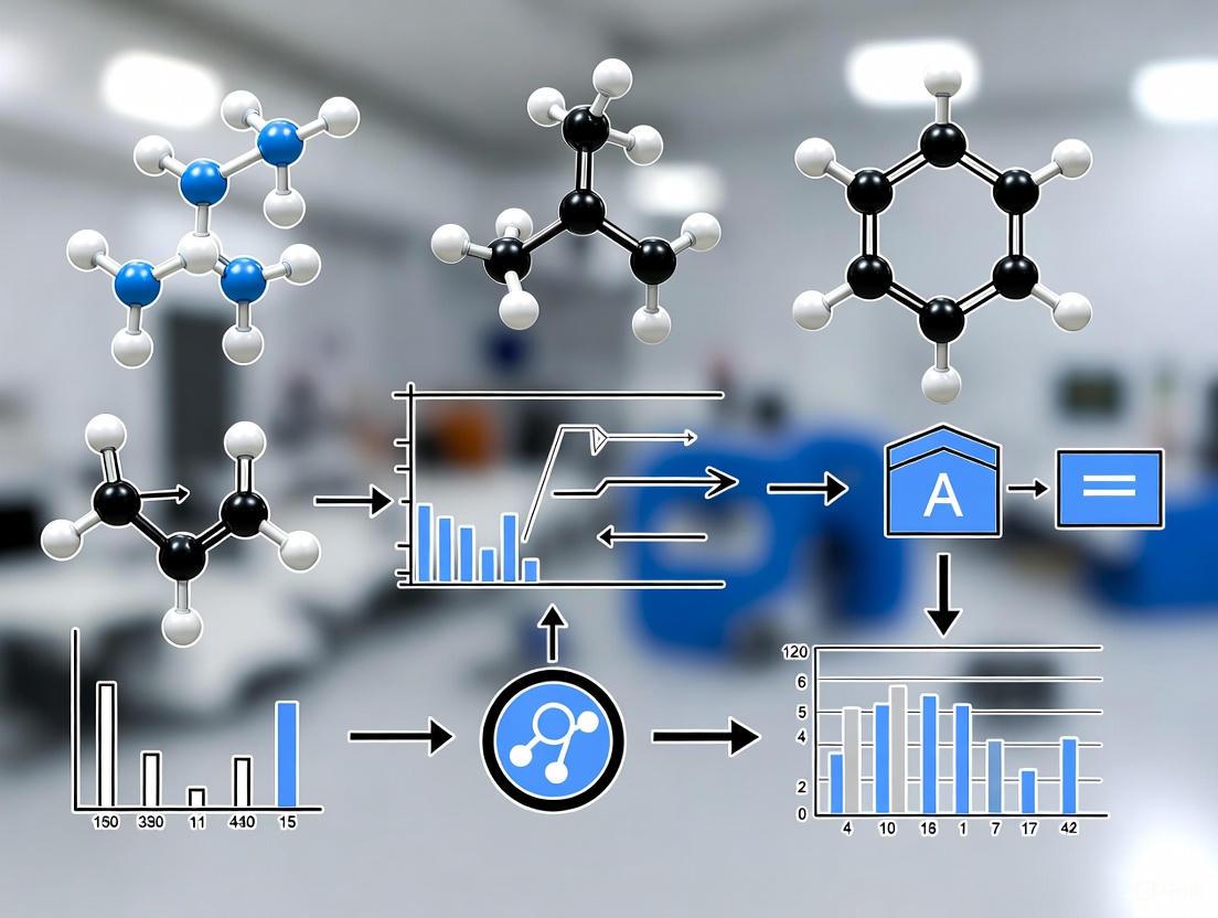
For researchers requiring robust, post-processing solutions, advanced deep-learning techniques are showing promise. For example, the CLEnet algorithm integrates a dual-scale Convolutional Neural Network (CNN) with Long Short-Term Memory (LSTM) networks and an improved attention mechanism [5]. This architecture is designed to extract both the morphological and temporal features of EEG, enabling it to separate clean EEG from artifacts even in multi-channel data containing "unknown" artifact types. One study reported that CLEnet improved the Signal-to-Noise Ratio (SNR) by 2.45% and decreased the relative root mean square error in the temporal domain (RRMSEt) by 6.94% [5].
The workflow for implementing such a modern artifact removal pipeline is outlined below.
The Scientist's Toolkit: Key Research Reagents & Materials
Table 3: Essential Materials for Few-Channel EEG Research
| Item | Function & Importance |
|---|---|
| Portable EEG Amplifier | The core hardware for signal acquisition. Key specifications for few-channel work include high input impedance (for dry electrodes), good common-mode rejection ratio (to reject environmental noise), and low intrinsic noise [6] [1]. |
| Dry or Semi-Wet Electrodes | Enable rapid setup and improve participant comfort for long-term, ambulatory recordings. Their use is a primary factor defining wearable EEG but requires careful management of impedance [1]. |
| Conductive Gel & Abrasion Kits | For wet electrode systems, proper skin preparation and low-impedance gel are critical for obtaining a stable signal and preventing electrode pops [4]. |
| Electrode Cap/Headset | The physical interface. A secure, well-fitting cap is essential to minimize motion artifacts. Material and design should be chosen for the target population and recording environment. |
| Auxiliary Sensors (IMU, EOG, EMG) | Inertial Measurement Units (IMUs) can track head movement, providing a reference signal for motion artifact correction. Dedicated EOG and EMG channels provide pristine reference signals for removing ocular and muscle artifacts, overcoming the limitations of few-channel source separation [1]. |
| Advanced Analysis Software | Software supporting modern techniques like deep learning (CLEnet [5]), wavelet transforms, or ICA [3] [1] is necessary for effective artifact management beyond simple filtering. |
For researchers working with few-channel portable EEG systems, achieving a high signal-to-noise ratio is a fundamental challenge. The data is invariably contaminated by artifacts—electrical signals generated from non-cerebral sources. These artifacts can obscure genuine neural activity and lead to misinterpretation of data. This technical support center provides a structured taxonomy of the primary artifact types—Motion, Ocular, Myogenic, and Technical—and offers evidence-based, practical troubleshooting guides framed within the context of contemporary artifact removal research for portable EEG systems.
Artifact Taxonomy & Identification Guide
The first step in effective artifact removal is accurate identification. The table below summarizes the core characteristics of the four main artifact categories.
Table 1: Taxonomy and Key Identifiers of Common EEG Artifacts
| Artifact Category | Primary Sources | Key Characteristics in EEG | Most Affected Frequency Bands |
|---|---|---|---|
| Motion Artifacts | Head movement, electrode displacement, cable sway [7] [8] [9] | Slow drifts, sharp amplitude bursts time-locked to gait cycle (e.g., heel strike), periodic oscillations [8] [9] | Delta, Theta [8] |
| Ocular Artifacts | Eyeblinks, eye movements (saccades) [10] [11] | High-amplitude, low-frequency signals; characteristic frontally-dominant topography [12] [10] | Delta (0.5-2 Hz) [12] |
| Myogenic Artifacts | Muscle activity in face, jaw, neck, and head [7] [10] | High-frequency, non-stationary, erratic waveform patterns [7] [10] | Beta, Gamma ( > 30 Hz) [7] |
| Technical Artifacts | Power line interference, faulty electrode contact, equipment limitations [8] | 50/60 Hz steady oscillation; "electrode pops" appear as sudden, large deflections [7] [8] | Specific to noise source (e.g., 60 Hz) |
Frequently Asked Questions (FAQs) for Researchers
Q1: Our gait study shows strong rhythmic noise during running. What preprocessing steps can we takebeforeICA to improve source separation?
A: Motion artifacts during running can overwhelm ICA. Two effective preprocessing methods are:
- iCanClean: This method uses canonical correlation analysis (CCA) to identify and subtract noise subspaces from the EEG signal. It can use dedicated noise sensors or create "pseudo-reference" signals from the EEG itself (e.g., by notch-filtering below 3 Hz to isolate motion noise). Studies show it significantly reduces power at the gait frequency and its harmonics, leading to better ICA decomposition with more dipolar brain components [13] [9].
- Artifact Subspace Reconstruction (ASR): ASR uses a sliding-window PCA to identify and remove high-variance signal components that deviate from a clean calibration period. An aggressive but effective
kparameter of 10 is recommended for locomotion studies to avoid over-cleaning while still mitigating motion artifacts [9].
Q2: For our portable single-channel EEG system, how can we effectively remove eyeblink artifacts without multiple channels for ICA?
A: Multi-channel methods like ICA are not suitable for single-channel data. Instead, consider data-driven decomposition approaches:
- Fixed Frequency Empirical Wavelet Transform (FF-EWT): This recent method adaptively decomposes the single-channel signal into components (IMFs). Components contaminated by EOG artifacts can be automatically identified using metrics like kurtosis, dispersion entropy, and power spectral density, and then removed with a specialized filter (e.g., GMETV). This method is designed to preserve essential low-frequency brain activity while targeting the 0.5-12 Hz range of eyeblink artifacts [12].
- Singular Spectrum Analysis (SSA): SSA is a subspace-based technique that can separate low-frequency oscillating noise, like EOG, from monovariate signals. Its performance can be improved with automated thresholding based on diffusion entropy [12].
Q3: We detect high-frequency noise in our forehead channels. Is this muscle or motion artifact?
A: This is most likely myogenic (muscle) artifact. Muscle contractions from the forehead, jaw, or scalp produce high-frequency, non-stationary, and erratic signals that are most prominent in the Beta and Gamma bands [7] [10]. In contrast, motion artifacts from head movement typically manifest as lower-frequency drifts or bursts time-locked to movement [8]. The Optimized Fingerprint Method uses a machine-learning model trained on features like spectral properties to automatically classify and remove such myogenic components from ICA decompositions [10].
Experimental Protocols for Artifact Removal
Protocol 1: ICA-based Removal of Ocular Artifacts in Free-Viewing Paradigms
This protocol is optimized for experiments where participants freely view stimuli, generating many eye movements [11].
Workflow Overview:
Detailed Methodology:
- Data Acquisition: Simultaneously record EEG and eye-tracking data.
- Filtering: Apply optimal high-pass (e.g., 2 Hz) and low-pass (e.g., 40-60 Hz) filters to the training data for ICA. This filtering step is critical for improving the quality of the ICA decomposition [11].
- Training Data Selection: Massively overweight the proportion of training data that contains myogenic saccadic spike potentials (SPs). This ensures the ICA algorithm is finely tuned to isolate these artifacts [11].
- Component Rejection: Use the synchronized eye-tracking data to objectively set thresholds for rejecting artifact-related independent components, minimizing both under-correction and over-correction [11].
Protocol 2: Deep Learning for Subject-Specific Motion Artifact Removal
This protocol uses a convolutional neural network (CNN) for end-to-end artifact removal, ideal for mobile EEG (mo-EEG) where artifact patterns are highly variable [8].
Workflow Overview:
Detailed Methodology:
- Model Architecture: Implement Motion-Net, a 1D CNN based on a U-Net architecture, which is effective for signal reconstruction tasks [8].
- Feature Engineering: Extract Visibility Graph (VG) features from the EEG signals. These features convert the time-series into a graph network, capturing non-linear structural properties that enhance the model's learning, especially on smaller datasets [8].
- Subject-Specific Training: Train and test the model on a per-subject basis. This approach accounts for individual variability in both brain signals and motion artifact patterns, leading to more robust performance than generalized models. The model is trained using real EEG recordings with ground-truth references (e.g., from static conditions) [8].
- Output: The model outputs a cleaned EEG signal. This approach has demonstrated an average motion artifact reduction of 86% and a significant improvement in Signal-to-Noise Ratio (SNR) [8].
The Scientist's Toolkit: Key Algorithms & Methods
Table 2: Essential "Research Reagent" Solutions for Artifact Removal
| Tool/Method | Primary Function | Key Advantage for Few-Channel EEG |
|---|---|---|
| iCanClean [13] [9] | Preprocessing of motion artifacts | Effective with pseudo-reference noise signals derived from EEG itself; improves subsequent ICA. |
| Artifact Subspace Reconstruction (ASR) [9] | Preprocessing of high-amplitude artifacts | Cleans data in real-time or offline before ICA; works on continuous data. |
| Fixed Frequency EWT (FF-EWT) [12] | Single-channel ocular artifact removal | Data-driven decomposition without needing reference channels. |
| Optimized Fingerprint Method [10] | Automatic classification of artifact components in ICA | Uses a tailored set of spatial, temporal, spectral, and statistical features for each artifact type. |
| Motion-Net (CNN) [8] | Subject-specific motion artifact removal | Does not rely on ICA; powerful for modeling complex, non-linear artifact patterns. |
The Impact of Dry Electrodes and Reduced Scalp Coverage on Signal Quality
The advancement of electroencephalography (EEG) towards portable, user-friendly, and long-term monitoring systems has driven the adoption of dry electrodes and reduced-channel arrays. These technologies are pivotal for applications in brain-computer interfaces, neuro-monitoring in drug development, and real-world cognitive studies. However, their impact on signal quality presents a significant challenge for researchers. Dry electrodes, while eliminating the preparation time and discomfort of conductive gels, are often more susceptible to motion artifacts and higher impedance. Similarly, reducing the number of electrodes compromises spatial resolution and can lower sensitivity to certain neural events. This technical support center provides evidence-based troubleshooting and FAQs to help researchers mitigate these challenges within the context of artifact removal for few-channel portable EEG systems.
Performance Data & Experimental Protocols
Quantitative Impact on Signal Acquisition
The following tables summarize key quantitative findings on how dry electrodes and reduced scalp coverage impact signal quality and operational performance.
Table 1: Impact of Reduced Electrode Arrays on Seizure Detection Sensitivity
| Study Reference | Number of EEG Channels | Seizure Type | Sensitivity | Specificity |
|---|---|---|---|---|
| [14] | 7 (Reduced Array) | Any Seizure | 70% | 96% |
| [14] | 7 (Reduced Array) | Focal Seizures | 80% | Not Specified |
| [14] | 7 (Reduced Array) | Generalized Seizures | 55% | Not Specified |
| [14] | 7 (Reduced Array) | Encephalopathic Patterns | 62% | 86% |
| [15] | 12 (Reduced Dry Array) | Neonatal Seizures | High (Correlation >0.8 with wet systems) | Not Specified |
Table 2: Dry vs. Wet Electrodes and Signal Quality Metrics
| Electrode Type | Key Advantages | Key Challenges & Signal Quality Impact | Best for Experimental Scenarios |
|---|---|---|---|
| Wet (Passive) | Excellent signal quality, low noise, stable impedance [16] | Long setup time, patient discomfort, gel can dry out [15] | Clinical diagnostics, high-fidelity lab studies |
| Dry (Passive) | Rapid setup, no gel, high patient comfort [16] | Higher impedance, more susceptible to motion artifacts [17] [15] | Short-term BCI, rapid screening, field studies |
| Active Dry | On-board amplification, superior noise immunity, good signal strength [15] | Higher cost, more complex design, requires power [15] | Long-term monitoring, movement-heavy paradigms |
Key Experimental Protocols from Literature
Protocol 1: Validating a Reduced Electrode Array for Inpatient Seizure Detection [14]
- Objective: To evaluate the sensitivity and specificity of a 7-electrode array for detecting seizures in hospitalized adults.
- Methodology:
- Data Collection: Retrospectively selected 100 EEG records (50 ictal, 50 non-ictal) from inpatients.
- Lead Reduction: Full 10-20 system recordings were digitally processed to simulate a 7-lead array (F3, F4, T7, T8, Cz, O1, O2).
- Blinded Review: Two epileptologists independently reviewed the reduced-array traces, documenting seizures and background disturbances.
- Analysis: Compared reviewers' findings to the original formal EEG report (the gold standard) to calculate sensitivity and specificity.
Protocol 2: Assessing a Novel Dry-Electrode Headset for Neonatal Seizure Monitoring [15]
- Objective: To develop and test a low-cost, adjustable headset with active dry-contact electrodes for continuous neonatal EEG.
- Methodology:
- Hardware Design: Created a 12-channel headset with 3D-printed, adjustable components and Ag/AgCl multi-spike electrodes.
- Signal Acquisition: Incorporated active electrodes with on-board buffering to strengthen signals and mitigate noise.
- Clinical Validation: Conducted simultaneous recordings on a pediatric patient using the custom dry-electrode device and a commercial wet-electrode system.
- Analysis: Computed cross-correlation and Signal-to-Noise Ratio (SNR) to compare signal quality between the two systems.
Protocol 3: Combining Spatial and Temporal Denoising for Dry EEG [17]
- Objective: To investigate if combining Independent Component Analysis (ICA)-based methods (Fingerprint+ARCI) with spatial filtering (SPHARA) improves dry EEG signal quality.
- Methodology:
- Data Recording: Recorded 64-channel dry EEG from 11 healthy volunteers during a motor execution paradigm.
- Processing Pipeline: Applied multiple denoising approaches: ICA-based methods alone, spatial filtering alone, and a combination of both.
- Quality Metrics: Quantified signal quality using Standard Deviation (SD), Signal-to-Noise Ratio (SNR), and Root Mean Square Deviation (RMSD).
- Statistical Analysis: Used a generalized linear mixed effects (GLME) model to identify significant changes in signal quality parameters.
Troubleshooting Guides & FAQs
Frequently Asked Questions
Q1: My dry-electrode EEG data has a high noise floor. What are the first steps I should take?
- A: First, verify electrode-scalp contact. Ensure the headset is snug and all electrodes are making firm contact, particularly through hair. Second, check for environmental noise sources and increase the distance from power cables or monitors. Third, if using passive dry electrodes, consider switching to active dry electrodes, which incorporate a high-input-impedance amplifier directly at the electrode site to buffer the signal and drastically reduce noise [15].
Q2: I am using a reduced channel setup (e.g., 3 channels). How can I compensate for the lost spatial information?
- A: Leverage advanced feature extraction and deep learning methods that enrich the temporal and spectral information from the few available channels. One effective method is to create a Channel-Dependent Multilayer EEG Time-Frequency Representation (CDML-EEG-TFR). This involves converting each channel's signal into a 2D time-frequency image using Continuous Wavelet Transform and then stacking these images to create a rich, multi-dimensional input that allows deep learning models to learn integrated spatio-spectro-temporal features [18].
Q3: My analysis is confounded by physiological artifacts (e.g., blinks, muscle noise). What is a robust denoising pipeline for dry EEG?
- A: A combination of temporal and spatial techniques has been shown to be highly effective. A recommended pipeline is:
- ICA-based Correction: Use methods like Fingerprint and ARCI to identify and remove components corresponding to ocular and muscle artifacts [17].
- Spatial Filtering: Apply a spatial method like Spatial Harmonic Analysis (SPHARA) as a subsequent step. This combination has been proven to yield superior noise reduction and lower signal deviation in dry EEG data compared to either method alone [17].
Q4: Is a reduced electrode array sufficient for detecting pathological patterns like seizures?
- A: Caution is advised. While specificity can remain high (>95%), sensitivity can drop significantly. One study found a 7-electrode array had only 70% sensitivity for detecting any seizure, with performance varying by seizure type (80% for focal, 55% for generalized) [14]. The clinical or research objective must guide this decision: reduced arrays may be useful for screening, but a full array is recommended for definitive diagnosis or comprehensive analysis.
Troubleshooting Common Recording Failures
Problem: Unstable or Grayscale Impedance Readings on Multiple Channels.
- Possible Cause & Solution: This often indicates a ground or reference electrode issue.
- Action 1: Re-apply the ground (GND) and reference (REF) electrodes. Ensure thorough skin preparation (cleaning and mild abrasion).
- Action 2: Try an alternative GND placement, such as the mastoid, forearm, or sternum.
- Action 3: Systematically test components (headbox, amplifier) to isolate the fault. A problem that persists across different system components likely originates with the participant or electrode connections [4].
Problem: Excessive High-Frequency Noise in the Signal.
- Possible Cause & Solution: This is frequently caused by high electrode-skin impedance, often with dry electrodes.
- Action 1: Readjust the headset and check for poor electrode-scalp contact.
- Action 2: Ensure the subject is relaxed, as muscle tension (EMG) is a common source of high-frequency noise. Its frequency range (0 to >200 Hz) can broadly contaminate EEG signals [3].
- Action 3: For dry systems, confirm that the design includes active shielding and driven-right-leg (DRL) circuits to suppress common-mode noise [15].
The Scientist's Toolkit
Table 3: Essential Research Reagents & Materials for Few-Channel Dry EEG Research
| Item Name | Function & Explanation |
|---|---|
| Active Dry-Contact Electrodes | Electrodes with integrated high-input-impedance amplifiers. They buffer the weak EEG signal at the source, combating the high impedance and motion artifacts typical of dry systems [15]. |
| Adjustable 3D-Printed Headset | A customizable headset platform that ensures stable and consistent electrode placement across different head sizes and shapes, which is critical for reproducible results with reduced arrays [15]. |
| Blind Source Separation (BSS) Software | Software packages (e.g., implementing ICA) are crucial for decomposing multi-channel EEG data to isolate and remove artifact-laden components from brain signals [3]. |
| Continuous Wavelet Transform (CWT) Toolbox | A computational tool for creating time-frequency representations of single-channel EEG data. This is a key step in creating enriched feature sets (like CDML-EEG-TFR) for few-channel analysis [18]. |
| Spatial Filtering Algorithms (e.g., SPHARA) | Algorithms that leverage the spatial geometry of the electrode array to suppress noise and enhance the signal-to-noise ratio, complementing temporal filtering methods [17]. |
Workflow & Signaling Diagrams
Dry EEG Signal Acquisition and Processing
Reduced-Channel EEG Analysis Pathway
FAQs & Troubleshooting Guides
This section addresses frequently encountered challenges and questions in mobile EEG research, providing targeted solutions for artifact management in real-world studies.
Frequently Asked Questions
Q: What are the most effective preprocessing methods for removing motion artifacts during high-movement activities like running?
- A: Research comparing motion artifact removal approaches during overground running indicates that iCanClean and Artifact Subspace Reconstruction (ASR) are highly effective. iCanClean, which uses canonical correlation analysis (CCA) with pseudo-reference noise signals derived from the EEG data itself, has been shown to be somewhat more effective than ASR in recovering brain components and restoring expected event-related potential (ERP) patterns, such as the P300 effect, during running [9].
Q: How can I identify and remove eye-blink (EOG) artifacts from a single-channel EEG recording?
- A: For single-channel systems, an automated method using Fixed Frequency Empirical Wavelet Transform (FF-EWT) combined with a GMETV filter has been demonstrated as effective [12]. The FF-EWT decomposes the signal, and components contaminated with EOG artifacts are identified using metrics like kurtosis, dispersion entropy, and power spectral density. These artifact-related components are then removed using the GMETV filter, which helps preserve essential low-frequency EEG information [12].
Q: Our research involves participants walking in real-world environments. How can we maintain data quality without being on-site to fix issues?
- A: Establishing robust remote troubleshooting protocols is key.
- Familiarize Staff: Ensure all researchers are deeply familiar with the equipment to give clear, specific instructions to on-site assistants or participants via phone [19].
- Leverage Software Tools: Use software features to hide severely affected channels or adjust sensitivity and filters on-the-fly to mitigate the impact of poor electrode contacts without permanently altering the raw data [19].
- Define Clear Protocols: Create and follow pre-established criteria for different scenarios (e.g., when to contact on-call staff for electrode re-application) to ensure consistent and timely responses to data quality issues [19].
- A: Establishing robust remote troubleshooting protocols is key.
Q: What steps should we take if we experience significant technical interference or connectivity issues during a remote monitoring session?
- A: Technical issues require a systematic approach [19]:
- Document the Issue: Note the time and nature of the problem.
- Follow Known Solutions: If it is a known issue with a documented workaround, implement it.
- Escalate to IT: If the issue is unresolved, contact the relevant IT support (e.g., hospital IT for facility-side issues).
- Utilize Leadership Chain: Exhaust all resources and escalate within your team's leadership to liaise with facility leadership and IT for a permanent fix.
- A: Technical issues require a systematic approach [19]:
Q: How should I prepare a participant for a long-term, in-home EEG recording to minimize artifacts?
- A: Proper participant preparation is crucial for data quality [20]:
- Hygiene: Instruct the participant to shampoo their hair within 24 hours of the appointment without using any products (spray, oil, gel) afterward.
- Clothing: Advise them to wear a button-down or zippered shirt to avoid pulling off electrodes when changing.
- Activity Restrictions: Clearly state that they must avoid extreme physical activity (running, jumping, swimming), gum chewing, and consuming hard candy for the duration of the recording.
- Environment: Prepare a clear, flat surface in a well-ventilated area for the EEG equipment setup.
- A: Proper participant preparation is crucial for data quality [20]:
Methodologies & Performance Data
This section provides detailed protocols and quantitative performance metrics for key artifact removal techniques relevant to mobile EEG research.
Table 1: Motion Artifact Removal Performance During Running
The following table summarizes the effectiveness of two prominent approaches for cleaning motion artifacts from EEG data recorded during overground running, based on a comparative study [9].
| Approach | Key Mechanism | Key Parameters | Performance on Running Data |
|---|---|---|---|
| Artifact Subspace Reconstruction (ASR) | Uses a sliding-window PCA to identify and remove high-variance components based on a clean calibration period [9]. | k threshold: Standard deviation threshold for artifact identification. A lower k is more aggressive. k=20-30 is often recommended, but k=10 may be needed for running to avoid overcleaning [9]. | Reduced power at gait frequency; produced ERP components similar to standing tasks [9]. |
| iCanClean | Employs Canonical Correlation Analysis (CCA) to identify and subtract noise subspaces highly correlated with pseudo-reference noise signals [9]. | R² threshold: Correlation criterion for noise subtraction. R²=0.65 with a 4s sliding window is effective for running data [9]. | Most effective at reducing gait-frequency power; recovered expected P300 congruency effect; produced the most dipolar brain ICs [9]. |
Table 2: Single-Channel Artifact Removal Techniques
This table compares methods designed for artifact removal when only a single EEG channel is available.
| Artifact Type | Technique | Protocol Summary | Reported Outcome |
|---|---|---|---|
| Eye-blink (EOG) | Fixed Frequency EWT + GMETV Filter [12] | 1. Decompose signal via FF-EWT into 6 IMFs.2. Identify artifact components using kurtosis, dispersion entropy, and PSD thresholds.3. Apply GMETV filter to remove artifact components. | Lower RRMSE, higher CC on synthetic data; improved SAR and MAE on real EEG [12]. |
| General (Ocular, Muscular, Movement) | Adaptive Wavelet-Based Renormalization [21] | A data-driven renormalization of wavelet components to adaptively attenuate artifacts of different natures. | Showed superior performance across various artifacts and signal-to-noise levels compared to alternative techniques [21]. |
Experimental Protocol: Validating Mobile EEG with Augmented Reality
This protocol outlines a methodology for studying cognition in real-world mobile settings while maintaining experimental control, using a combination of mobile EEG and Augmented Reality (AR) [22].
- Objective: To validate the use of mobile EEG in free-moving conditions combined with AR by replicating the well-established face inversion effect (greater low-frequency EEG activity for inverted vs. upright faces) [22].
- Equipment:
- EEG: 64-channel mobile EEG system (e.g., BrainVision LiveAmp) with active electrodes.
- AR: Head-mounted AR display (e.g., Microsoft Hololens 2).
- Video: Head-mounted camera for scene recording and event tagging.
- Procedure:
- Task 1 (Lab Control): Participants view upright and inverted faces on a computer screen while seated to establish a baseline neural response.
- Task 2 (Mobile with Photos): Participants walk through a corridor and view physical photographs of upright and inverted faces attached to the walls, pressing a button to tag viewing events.
- Task 3 (Mobile with AR): Participants walk through the same corridor wearing the AR headset, viewing virtual 3D faces anchored to the environment, and tag events with a button press.
- Analysis:
- Epoch-based: EEG data is filtered (e.g., 1-20 Hz for mobile tasks), and epochs are extracted around face-viewing events. Power in the theta/low-alpha band (e.g., 4-10 Hz) is compared between upright and inverted conditions.
- Continuous GLM-based: A General Linear Model (GLM) is used to relate the continuous, dynamic EEG signal to the continuous stream of face perception states (upright vs. inverted) as the participant moves naturally.
- Validation: The study successfully identified the face inversion effect across all three tasks, demonstrating that cognitively relevant neural signals can be reliably measured using mobile EEG and AR paradigms [22].
The Scientist's Toolkit
This table lists essential computational tools and materials used in modern mobile EEG research for artifact removal and signal processing.
| Tool/Reagent | Function in Research |
|---|---|
| iCanClean | A signal processing toolbox designed to remove motion artifacts from mobile EEG by leveraging reference noise signals (from dedicated sensors or created pseudo-referentially) and Canonical Correlation Analysis (CCA) [9]. |
| Artifact Subspace Reconstruction (ASR) | An algorithm that uses a sliding-window principal components analysis (PCA) to identify and remove high-amplitude, non-stereotypical artifacts from continuous EEG data in real-time or during preprocessing [9]. |
| Fixed Frequency EWT (FF-EWT) | A signal decomposition technique that adaptively creates wavelet filters tuned to specific fixed frequencies, ideal for separating artifact-dominated components (like EOG) from neural signals in single-channel EEG [12]. |
| Independent Component Analysis (ICA) | A blind source separation method that linearly decomposes multi-channel EEG into maximally independent components, which can then be manually or automatically classified and removed if they represent artifacts [9]. |
| Mobile EEG System | A wearable, amplifier-based EEG system that allows for high-fidelity neural recordings while participants are freely moving. Often uses active electrodes and wireless data recording [22]. |
| Augmented Reality (AR) Headset | A head-mounted display that overlays virtual objects onto the real-world environment, enabling experimental control over visual stimuli in ecologically valid, real-world settings [22]. |
Workflow & System Diagrams
Signal Processing for Motion Artifact Removal
Mobile EEG-AR Experimental Workflow
Cutting-Edge Pipelines for Detection and Removal
Frequently Asked Questions (FAQs)
FAQ 1: Why should I choose VMD over the more traditional EMD for processing my single-channel EEG data?
VMD (Variational Mode Decomposition) possesses a robust mathematical foundation based on the variational principle, which transforms the decomposition problem into an optimization problem [23]. In contrast, EMD (Empirical Mode Decomposition) is often criticized for lacking a strong theoretical foundation and being more of a mathematical trick [23]. From a practical standpoint, VMD effectively overcomes the problem of modal mixing (aliasing) that frequently plagues EMD and can lead to data superposition in the decomposed components [24] [25]. Furthermore, VMD exhibits excellent noise robustness in practical applications, making it particularly suitable for the often noisy signals from portable EEG systems [25].
FAQ 2: How do I handle the critical parameter selection for VMD, specifically the number of modes (K)?
Selecting the correct number of intrinsic mode functions (IMFs), denoted as K, is indeed a crucial and challenging step for VMD [23]. An incorrect 'K' can lead to serious decomposition errors. While this often requires analysis of the specific signal, one practical approach is to start with a parameter optimization method. Research has successfully combined VMD with fuzzy entropy to identify artifact components after decomposition [25]. For a more automated solution, you can consider newer algorithms like QVMD (Queued Variational Mode Decomposition), which can determine the modal number adaptively during the separation process, eliminating the need for this prior information [23].
FAQ 3: My decomposed signal components show significant distortion at the endpoints. What is causing this and how can it be fixed?
This is a well-known challenge known as the "end effect," and it is not unique to one method—it can occur in EMD, EWT, and VMD [23]. The distortion arises because the decomposition algorithms have limited information at the signal boundaries. A common technique to mitigate this is to perform an end elongation of the composite signal before decomposition. For instance, the QVMD method uses a Principal Component Restoring (PCR) approach, which extracts trend lines and principal components from the end regions to effectively reduce the end effect to a much lower level [23].
FAQ 4: For my single-channel EEG artifact removal, which Blind Source Separation (BSS) method works best after signal decomposition?
Research indicates that the SOBI (Second Order Blind Identification) algorithm, an ICA implementation based on second-order statistics, is particularly effective for processing certain artifacts like EMG (electromyography) [24] [25]. While ICA methods based on high-order statistics are widely used, they are not as effective as SOBI for EMG artifacts [24] [25]. Therefore, for a method targeting multiple artifacts including EOG and EMG, a combination of VMD with SOBI has been shown to have a better removal effect compared to other combinations like EEMD-SOBI [24] [25].
FAQ 5: Are there readily available Python libraries to get started with these decomposition methods for my research?
Yes, several Python packages can help you implement these methods quickly. The PySDKit library provides a Scikit-learn-like interface for various signal decomposition algorithms, including EMD and VMD [26]. Specifically for EMD, the PyEMD package is available, which includes EEMD and CEEMDAN implementations [27]. For VMD and EWT, you can use the vmdpy and ewtpy packages, which have been used in comparative studies for EEG seizure detection [28].
Troubleshooting Guides
Issue 1: Poor Artifact Removal Performance in Single-Channel EEG
This guide addresses the problem of suboptimal artifact removal when using decomposition methods on a single EEG channel, which is common in portable systems.
- Symptoms: Useful brain signals are accidentally removed along with artifacts; artifacts persist in the reconstructed signal; reconstructed EEG signal appears overly smoothed or contains residual noise.
- Possible Causes & Solutions:
| Cause | Solution |
|---|---|
| Incorrect number of modes (K) in VMD | Optimize the K parameter. Start by over-specifying K and use a metric like fuzzy entropy [25] or correlation to identify and discard artifact-only components. |
| Ineffective BSS algorithm for target artifact | Switch the BSS method. For EMG artifacts, use SOBI instead of high-order statistics-based ICA [24] [25]. |
| Modal Mixing in EMD | Use an ensemble method like EEMD or CEEMDAN. These add controlled noise to create multiple derived signals, reducing mode mixing [23] [27]. |
| General performance plateau | Try a hybrid approach. Decompose with VMD, then apply SOBI to the set of IMFs to separate sources, before identifying and removing artifact components [24] [25]. |
Recommended Experimental Workflow: The diagram below illustrates a robust experimental protocol for single-channel EEG artifact removal, synthesizing recommendations from multiple studies.
Issue 2: Excessive Computational Time During Decomposition
This guide helps resolve impractically long processing times, which hinders experimental iteration and potential real-time application.
- Symptoms: Decomposition of a short signal segment takes several minutes or hours; computer becomes unresponsive during processing; unable to process large datasets in a feasible time.
- Possible Causes & Solutions:
| Cause | Solution |
|---|---|
| Using EEMD/CEEMDAN with many trials | Reduce the trials (ensemble number) parameter. Balance between performance and speed; even a lower number of trials can provide benefits [27]. |
| Sequential processing of multiple signals | Enable parallel processing. For EEMD, set the parallel flag to True and define the number of processes to utilize multiple CPU cores [27]. |
| High maximum mode number in EMD | Limit the max_imf parameter to stop decomposition after a set number of IMFs are extracted, preventing unnecessary iterations [27]. |
| VMD with high iteration count | Adjust VMD's convergence parameters (AbsoluteTolerance, RelativeTolerance) to allow for earlier stopping [29]. |
Performance Comparison of Decomposition Methods: The table below summarizes key characteristics, including relative speed, to help you choose the right method.
| Method | Key Principle | Strengths | Weaknesses | Relative Speed |
|---|---|---|---|---|
| EMD | Iterative sifting to extract IMFs [23] | Fully data-driven; intuitive | Modal mixing; end effect; no theoretical basis [23] | Medium [28] |
| EEMD | EMD on signal + multiple noise realizations [27] | Reduces mode mixing | High computational cost; residual noise [23] | Slow [28] |
| VMD | Variational optimization for mode extraction [24] | Robust theoretical basis; noise robustness [24] | Requires pre-setting mode number K [23] | Fast [28] |
| EWT | Adaptive wavelet filter bank [23] | Solid theoretical foundation | Empirical spectrum segmentation [23] | Very Fast [28] |
Issue 3: Effectively Isolating Specific Artifact Types (EOG vs. EMG)
This guide addresses the challenge of selectively removing different physiological artifacts, which have distinct characteristics.
- Symptoms: Muscle artifacts (EMG) remain after removing eye-blink artifacts (EOG); removing EMG artifacts also degrades high-frequency brain signals (e.g., gamma waves).
- Possible Causes & Solutions:
| Cause | Solution |
|---|---|
| Using the same BSS method for all artifacts | Employ a specialized BSS. SOBI (SOS-based) is particularly effective for the characteristic profiles of EMG artifacts [24] [25]. |
| Incorrect identification of artifact components | Use a quantitative identification metric. Calculate the fuzzy entropy of each component; artifact components often have significantly different entropy values compared to neural signals [25]. |
| Overlapping frequency content | Leverage joint decomposition-separation. Rely on the source separation step (SOBI/ICA) after decomposition to statistically disentangle sources even with overlapping frequencies [24]. |
Logical Decision Tree for Artifact Isolation: The following diagram provides a step-by-step strategy for tackling mixed artifacts.
The Scientist's Toolkit: Research Reagent Solutions
Essential Computational Tools and Datasets
| Tool Name | Type / Function | Role in the Experimental Pipeline |
|---|---|---|
| PySDKit [26] | Python Library | Provides a unified Scikit-learn-like API for EMD, VMD, and other decomposition methods, streamlining the analysis workflow. |
| vmdpy & ewtpy [28] | Python Packages | Dedicated, validated implementations of VMD and EWT, ensuring reliable and reproducible decomposition results. |
| PyEMD [27] | Python Library | A comprehensive suite for Empirical Mode Decomposition and its variants (EEMD, CEEMDAN). |
MATLAB vmd [29] |
MATLAB Function | The official implementation of VMD in MATLAB, offering extensive parameters for fine-tuning the decomposition. |
| Public EEG Datasets (e.g., Bonn, NSC-ND) [28] | Benchmark Data | Essential for validating new artifact removal algorithms against established benchmarks and comparing performance. |
Key Performance Metrics for Method Validation When comparing the efficacy of different decomposition pipelines for artifact removal, quantify performance using these standard metrics, derived from semi-simulation experiments [25]:
| Metric | Definition | Ideal Outcome |
|---|---|---|
| Signal-to-Artifact Ratio (SAR) | Ratio of power in neural signal to power in artifact component. | Maximize |
| Root Mean Square Error (RMSE) | Difference between cleaned signal and ground-truth clean signal. | Minimize |
| Correlation Coefficient | Linear correlation between cleaned signal and ground-truth clean signal. | Maximize (Close to 1) |
| Spectral Distortion | Measure of unwanted changes in the frequency spectrum of the clean signal. | Minimize |
Frequently Asked Questions (FAQs)
Q1: What is the main advantage of using a subject-specific model like Motion-Net over a generalized model for motion artifact removal? Subject-specific models are trained and tested on data from individual users separately. This approach accounts for the high variability in both EEG signals and motion artifact patterns across different individuals, leading to significantly better performance. The Motion-Net framework has demonstrated an average motion artifact reduction of 86% ±4.13 and a signal-to-noise ratio (SNR) improvement of 20 ±4.47 dB, outperforming generalized models which struggle with inter-subject variability [30].
Q2: My dataset is relatively small. Can I still effectively train a deep learning model for artifact removal? Yes, incorporating specific features can enhance model performance on smaller datasets. Motion-Net successfully uses Visibility Graph (VG) features, which convert time-series EEG data into graph structures, providing additional structural information that helps the Convolutional Neural Network (CNN) learn more effectively even with limited data [30]. Other studies also use data augmentation techniques, such as adding noise or sliding window sampling, to artificially increase the size of the training set [31].
Q3: For a portable EEG system with only a few channels, which deep learning architecture is most suitable? Architectures designed for 1D signal processing, such as 1D CNNs, are particularly well-suited for few-channel systems. Motion-Net employs a 1D U-Net architecture, which is effective for signal reconstruction tasks [30]. Similarly, other research uses a 1D-ResCNN (Residual CNN) or combines dual-scale CNNs with LSTM networks (e.g., CLEnet) to capture both morphological and temporal features from multi-channel data, even with a limited number of electrodes [32] [33].
Q4: How do I handle different types of artifacts (e.g., eye blinks, muscle activity) with a single model? While some models are tailored for specific artifacts, newer architectures aim for generalization. For instance, the CLEnet model, which integrates CNN and LSTM layers, has shown proficiency in removing various artifacts, including EMG, EOG, and even "unknown" artifacts in multi-channel EEG data, by leveraging an improved attention mechanism to extract robust features [33]. However, achieving high performance across all artifact types with one model remains an active research challenge.
Troubleshooting Guides
Issue 1: Poor Artifact Removal Performance on New Subjects
Problem: Your model, which performed well during training, fails to generalize to data from new subjects.
Solutions:
- Adopt a Subject-Specific Approach: Retrain the model separately for each subject using their own data. This is the core methodology of Motion-Net and avoids the problem of inter-subject variability [30].
- Incorplement Advanced Features: Augment your raw EEG input with engineered features like the Visibility Graph (VG), which can improve the model's learning stability and accuracy, particularly with smaller, subject-specific datasets [30].
- Use Domain Adaptation: Explore self-supervised learning techniques that can help the model adapt to new subjects or sessions with minimal labeled data. Methods like contrastive learning and masked prediction tasks can learn robust features that are less dependent on the individual [34].
Issue 2: Low Signal-to-Noise Ratio in Portable EEG Recordings
Problem: The input EEG data from your portable device has a very low SNR, making it difficult for the model to distinguish artifacts from neural signals.
Solutions:
- Pre-process with Filtering: Apply band-pass filters to remove frequency components outside the range of interest (e.g., 1-100 Hz for EEG). However, be cautious as motion artifacts often overlap with neural signal frequencies [30].
- Leverage Multi-Modal Data: If available, use data from integrated accelerometers or gyroscopes to independently detect motion events. This information can be synchronized with EEG data to improve artifact identification [30].
- Choose a Robust Model Architecture: Implement models specifically designed for noisy signals. For example, the AnEEG model uses a Generative Adversarial Network (GAN) with LSTM layers to capture temporal dependencies and generate artifact-free signals, even from highly contaminated data [32].
Issue 3: Model Training is Unstable or Fails to Converge
Problem: During the training of your CNN model, the loss function fluctuates wildly or does not decrease.
Solutions:
- Inspect and Pre-process Data: Ensure your data is properly synchronized and that a baseline correction (e.g., polynomial deduction) has been applied. Check for extreme outliers or non-physiological noise that could destabilize training [30].
- Adjust Hyperparameters: Tune key parameters such as learning rate and batch size. Using an adaptive learning rate scheduler can help. For optimal performance, consider using hyperparameter optimization frameworks like Optuna [35].
- Review Loss Functions: For reconstruction tasks, standard losses like Mean Squared Error (MSE) are common. Some studies, particularly those using GANs, employ advanced loss functions that incorporate temporal-spatial-frequency constraints to better guide the training process [32].
The table below summarizes the performance metrics of several deep learning models for EEG artifact removal, as reported in the search results.
| Model Name | Architecture Type | Primary Application | Key Performance Metrics |
|---|---|---|---|
| Motion-Net [30] | 1D U-Net CNN | Motion Artifact Removal | Artifact reduction (η): 86% ±4.13SNR improvement: 20 ±4.47 dBMAE: 0.20 ±0.16 |
| CLEnet [33] | Dual-scale CNN + LSTM | Multi-artifact Removal (EMG, EOG) | SNR: 11.498 dBCC: 0.925RRMSEt: 0.300 |
| AnEEG [32] | LSTM-based GAN | General Artifact Removal | Improved SNR and SAR values; lower NMSE and RMSE compared to wavelet techniques. |
| 1D-ResCNN [31] | 1D Residual CNN | Eye Blink Artifact Removal | Outperformed ICA and regression methods, particularly for central head electrodes. |
Experimental Protocols & Methodologies
Protocol 1: Implementing a Subject-Specific Motion-Net Framework
This protocol is based on the methodology used to develop and validate the Motion-Net model [30].
Data Collection & Preprocessing:
- Collect EEG data using a portable system alongside a synchronized motion sensor (e.g., accelerometer).
- Record data during both resting states (to obtain clean "ground-truth" segments) and motion tasks (to create artifact-contaminated data).
- Synchronize EEG and accelerometer data by resampling and aligning them based on trigger points or event markers.
- Apply a baseline correction, such as deducting a fitted polynomial, to remove low-frequency drifts.
Feature Engineering & Input Formation:
- Extract Visibility Graph (VG) features from the EEG time series. This converts the signal into a graph representation that captures structural properties.
- Formulate the model input by combining raw EEG signals and the extracted VG features to provide complementary information.
Model Training & Validation:
- Design a 1D U-Net CNN architecture. The encoder should downsample to capture features, and the decoder should upsample to reconstruct the clean signal.
- Train the model on a per-subject basis. Use the artifact-contaminated signals as input and the corresponding clean segments or ground-truth references as the training target.
- Use a loss function like Mean Absolute Error (MAE) or Mean Squared Error (MSE) to minimize the difference between the output and the target clean signal.
- Validate the model using a separate, held-out dataset from the same subject.
Protocol 2: Training a Multi-Artifact Removal Model (CLEnet)
This protocol outlines the procedure for training an end-to-end model capable of handling various artifacts [33].
Dataset Preparation:
- Utilize a semi-synthetic dataset (e.g., from EEGdenoiseNet) where clean EEG is artificially contaminated with recorded EOG and EMG artifacts at known SNR levels.
- For real-world validation, use a dedicated multi-channel EEG dataset containing labeled or identifiable artifacts.
Model Architecture Setup:
- Implement a dual-branch network (CLEnet) that includes:
- A CNN branch with dual-scale convolutional kernels to extract morphological features at different scales.
- An LSTM branch to capture the temporal dependencies in the signal.
- An Improved EMA-1D (Efficient Multi-Scale Attention) module embedded in the CNN to enhance feature extraction and preserve temporal context.
- Implement a dual-branch network (CLEnet) that includes:
End-to-End Training:
- Train the model in a supervised manner using the contaminated EEG as input and the pristine, clean EEG as the target.
- Use MSE as the loss function to guide the reconstruction of the artifact-free signal.
- Evaluate the model on a test set using metrics such as SNR, Correlation Coefficient (CC), and Relative Root Mean Square Error (RRMSE).
The Scientist's Toolkit: Research Reagent Solutions
| Item / Technique | Function in Experiment |
|---|---|
| Visibility Graph (VG) Features [30] | Converts EEG time-series into graph structures, providing supplementary structural information that enhances deep learning model accuracy, especially with smaller datasets. |
| Synchronized Accelerometer Data [30] | Provides an independent measure of subject motion, used to validate and synchronize with motion artifacts in the EEG signal for improved identification and removal. |
| Semi-Synthetic Datasets (e.g., EEGdenoiseNet) [33] | Allows for controlled model training and benchmarking by providing clean EEG signals mixed with well-defined artifacts (EOG, EMG) at known signal-to-noise ratios. |
| Optuna Hyperparameter Optimization Framework [35] | An open-source library used to automatically search for and identify the optimal set of hyperparameters (e.g., learning rate, network depth) for a deep learning model. |
| Dual-Attention Mechanism [35] | A module integrated into neural networks (like MobileNetV2) that helps the model focus on the most relevant spatial and channel-wise features for the task, improving classification accuracy. |
| 1D U-Net Architecture [30] | A convolutional network architecture with a symmetric encoder-decoder structure, particularly effective for tasks involving signal reconstruction and segmentation, such as mapping noisy EEG to clean EEG. |
Experimental Workflow and Signaling Pathways
Motion-Net Experimental Workflow
Deep Learning Model Selection Logic
Core Concepts: How Auxiliary Sensors Capture Noise
Auxiliary sensors, such as IMUs and dual-layer EEG noise electrodes, provide independent measurements of motion and environmental interference that corrupt EEG signals. They act as reference channels, enabling sophisticated signal processing techniques to isolate and remove artifacts.
Dual-Layer EEG uses mechanically coupled but electrically isolated electrodes. The scalp layer records brain signals mixed with artifacts, while the noise layer records only non-biological artifacts (e.g., from cable movement or electromagnetic interference), providing a direct reference for cleaning the scalp data [36].
Inertial Measurement Units (IMUs) are motion sensors (accelerometers, gyroscopes) that directly quantify the kinematics of the head or body. This data serves as a reference for motion artifacts introduced into the EEG signal from physical movement [37] [38].
Table: Comparison of Auxiliary Sensor Types for Noise Reference
| Sensor Type | Primary Measured Noise | Spatial Resolution | Key Advantage | Common Use Case |
|---|---|---|---|---|
| Dual-Layer Noise Electrodes | Cable movement, electromagnetic interference, electrode-skin interface noise [36] | High (channel-level) | Directly captures electrical artifacts on the scalp; no additional head-worn sensors required [36]. | Whole-body movement studies (e.g., table tennis, walking) [36]. |
| Head-Mounted IMU | Gross head motion (acceleration, rotation) [37] | Low (system-level) | Directly measures the kinematics of the head; simple to implement [38]. | Mobile BCIs during walking, running [37]. |
| Per-Electrode IMU | Local electrode motion and displacement [38] | Very High (electrode-level) | Captures localized motion at each electrode; allows for targeted artifact removal [38]. | High-motion scenarios where different electrodes experience different artifacts. |
Frequently Asked Questions & Troubleshooting
Q1: The correlation between my IMU data and EEG channels is low. What could be wrong? Low correlation often stems from misalignment between the noise measured by the IMU and the artifact seen by the EEG electrode. Consider these points:
- Spatial Location: A single head-mounted IMU may not capture localized electrode movements effectively. Using a per-electrode IMU setup can provide a more accurate reference for each channel [38].
- Signal Type: The raw acceleration from an IMU might not be the best correlate of the electrical artifact. Try integrating the acceleration signal to derive velocity, which has been shown to correlate better with motion artifacts in some scenarios [38].
- Temporal Synchronization: Even minor misalignment between the EEG and IMU data streams can drastically reduce observed correlation. Ensure precise hardware synchronization or use post-hoc alignment based on a shared trigger or event [37].
Q2: When should I choose a dual-layer EEG system over a standard EEG with an IMU? The choice depends on the primary noise source in your experiment.
- Choose a Dual-Layer EEG system when the main artifacts are from cable sway, electrode movement, and electromagnetic interference. This system is specifically designed to reference these electrical artifacts directly [36].
- Use a Standard EEG with an IMU when the main artifacts are from gross head and body movements, and you have the processing pipeline to leverage the kinematic data for artifact removal [37].
Q3: I am working with few-channel, portable EEG. Which artifact removal method is most suitable? For few-channel systems, methods that can effectively leverage limited spatial information are key.
- Channel-Dependent Multilayer Time-Frequency Representations (CDML-EEG-TFR) can be a powerful approach. This method converts each channel's signal into a time-frequency image and stacks them, creating a rich input for deep learning models that can learn to disentangle brain activity from artifacts, even with few channels [18].
- Fine-tuned Large Brain Models (LaBraM) that incorporate IMU data have also shown robustness. These models can be adapted (fine-tuned) for few-channel scenarios, using the IMU's motion data to guide artifact removal with high efficiency [37].
Q4: After applying an artifact removal algorithm, I suspect it is also removing neural signals. How can I validate this? Validation is crucial. Beyond checking for improved signal-to-noise ratio, consider these strategies:
- Use a Task with Known Neurophysiology: Employ a paradigm with a well-established brain response (e.g., a visual evoked potential). If the cleaning algorithm preserves or enhances this known response, it indicates neural signals are retained [37].
- Check Component Topography: If using methods like ICA, inspect the topography of removed components. Components with a dipolar pattern that originates from brain-like regions are more likely to be neural and should be treated with caution [36] [3].
- Source Localization: Perform source localization on the data before and after cleaning. An effective algorithm should allow for more stable and physiologically plausible source estimates [39].
Experimental Protocols for Validation
Protocol 1: Validating Dual-Layer EEG Performance
Objective: To verify that the use of dual-layer noise electrodes provides cleaner brain components compared to single-layer processing [36].
Materials:
- Dual-layer EEG system (e.g., 120 scalp + 120 noise electrodes) [36].
- A paradigm inducing both neural activity and motion (e.g., table tennis drills or walking tasks).
Methodology:
- Data Collection: Record EEG data during the chosen paradigm using the dual-layer system. Ensure noise electrodes are electrically isolated but mechanically coupled to their corresponding scalp electrodes [36].
- Data Processing with Noise Reference: Process the data using the iCanClean algorithm or a similar approach (e.g., CCA) that explicitly uses the noise electrode data to identify and remove artifact components [36].
- Data Processing without Noise Reference: Process the same data using only the scalp channels and a standard artifact removal pipeline (e.g., ASR followed by ICA).
- Quantitative Comparison: For both processing streams, count the number of "high-quality" brain components after ICA. This is typically done by assessing the fit of a dipole model to each component and using an automated labeling algorithm. A higher number of brain components with a good dipole fit indicates superior preservation of neural signals [36].
Protocol 2: Benchmarking IMU-Enhanced Deep Learning
Objective: To evaluate the performance of a fine-tuned large brain model (LaBraM) using IMU data against a established benchmark (ASR-ICA) for motion artifact removal [37].
Materials:
- 32-channel EEG system.
- Head-mounted 9-axis IMU (3-axis accelerometer, gyroscope, magnetometer).
- A mobile BCI dataset with recordings from various movement conditions (standing, slow walking, fast walking, slight running) [37].
Methodology:
- Data Preprocessing: Preprocess the EEG signals (bandpass filter 0.1-75 Hz, notch filter at 60 Hz, resample to 200 Hz). Synchronize the IMU data with the EEG [37].
- Model Fine-Tuning: Use a pre-trained LaBraM model. Project both the EEG signals and the 9-axis IMU signals into a shared 64-dimensional latent space. Train a correlation attention mapping mechanism to allow the EEG queries to attend to relevant IMU keys for identifying motion artifacts. Fine-tune the model on approximately 5.9 hours of mobile EEG-IMU data [37].
- Benchmarking: Compare the fine-tuned LaBraM model's performance against the standard ASR-ICA pipeline. Evaluation should use metrics like Mean Squared Error (MSE) and Signal-to-Noise Ratio (SNR) on a held-out test set, and critically, the classification accuracy of the underlying BCI task (e.g., ERP classification) after artifact removal [37].
The Scientist's Toolkit: Essential Research Reagents & Materials
Table: Key Materials for Experimental Setup
| Item Name | Function / Application | Technical Notes |
|---|---|---|
| Dual-Layer EEG Cap | Records scalp EEG and mechanically-coupled noise references simultaneously. | Ensure noise electrodes are electrically isolated. 3D-printed couplers can be used to join scalp and noise electrodes [36]. |
| Active Electrodes with IMUs | Measures local electrode motion for data-driven artifact removal. | An IMU (accelerometer/gyroscope) is mounted directly on the PCB of each active electrode [38]. |
| 9-Axis Head-Mounted IMU | Provides reference signal for gross head motion (acceleration, rotation, orientation). | Often used as a single reference for the entire EEG system. Data can be integrated to derive velocity [37] [38]. |
| iCanClean Algorithm | A dual-layer processing method using CCA to reject components correlated with noise electrodes [36]. | An alternative to ICA-based approaches that explicitly uses the noise layer. |
| Artifact Removal Transformer (ART) | An end-to-end deep learning model (transformer-based) for denoising multichannel EEG [39]. | Trained on pseudo clean-noisy data pairs; can remove multiple artifact types simultaneously. |
| Mobile BCI Dataset | A public dataset containing synchronized EEG and IMU data from various motion states. | Used for training and benchmarking algorithms. Example: Mobile BCI dataset by Lee et al. with standing, walking, and running data [37]. |
Core Concepts and Challenges
What are the primary challenges in artifact removal for few-channel portable EEG systems that hybrid frameworks aim to solve?
Few-channel portable EEG systems, crucial for real-world applications like stroke rehabilitation and emotion recognition, face significant data quality challenges. Unlike high-density lab systems, they have limited spatial information and suffer from increased data sparsity, making traditional artifact removal methods less effective [18]. Furthermore, artifacts in these systems are diverse and often unknown or mixed (e.g., EMG, EOG, ECG), occurring simultaneously without reference channels, which challenges algorithms designed for single artifact types [40]. The signals are also inherently non-linear and non-stationary, contaminated by both physiological and non-physiological noise, requiring models that can capture complex temporal and morphological features [40] [41].
How do hybrid frameworks fundamentally differ from traditional signal processing for EEG artifact removal?
Traditional methods like Independent Component Analysis (ICA) or regression require manual intervention, struggle without reference signals, and often need a large number of channels [40]. Hybrid frameworks integrate the strengths of different deep learning architectures to create an end-to-end, automated solution. They combine models excelling in spatial feature extraction (like CNNs) with those capturing long-term temporal dependencies (like LSTMs), often enhanced with attention mechanisms to adaptively focus on the most salient features for robust, automated artifact removal even with few channels and unknown noise sources [40] [41].
Troubleshooting Guides & FAQs
FAQ 1: My hybrid model performs well on synthetic data but fails on real-world portable EEG data. What could be wrong?
This is a common issue known as the synthetic-to-real domain gap. The simulated artifacts in your synthetic dataset may not perfectly capture the complexity and variability of artifacts in authentic recordings.
- Troubleshooting Steps:
- Verify Data Synthesis: Critically review the methodology used to create your semi-synthetic data. Ensure the artifact-to-EEG mixing ratios reflect realistic scenarios. If possible, incorporate real artifacts recorded separately.
- Incorporate Real Data: Fine-tune your pre-trained model on a smaller dataset of real, artifact-contaminated EEG from your specific portable system. This adapts the model to the actual signal characteristics and noise profiles of your hardware.
- Use Data Augmentation: Apply robust data augmentation techniques during training to improve model generalization. For EEG, this can include channel reorganization, random noise injection, and signal transformation [34].
- Check Model Complexity: A model that is too complex might overfit to the patterns of your synthetic data. Consider simplifying the architecture or increasing regularization (e.g., dropout layers) to improve generalization to real data.
FAQ 2: How can I improve the performance of my hybrid model with very limited labeled training data?
This challenge is central to few-channel EEG research. Leveraging self-supervised and transfer learning is key to overcoming data sparsity.
- Troubleshooting Steps:
- Implement Self-Supervised Learning (SSL): Use methods like contrastive learning or masked prediction tasks on your large volume of unlabeled EEG data. For example, the EmoAdapt framework integrates both contrastive learning and masking to learn robust features from limited channels without needing extensive labels [34].
- Employ Transfer Learning: Utilize a pre-trained model from a related domain. One effective method is to convert few-channel EEG signals into a Channel-Dependent Multilayer Time-Frequency Representation (CDML-EEG-TFR). You can then use a pre-trained CNN (like EfficientNet) as a feature extractor, freezing its weights and training only a new classifier head. This transfers knowledge from large image datasets to your EEG analysis task [18].
- Data Augmentation: As above, aggressively augment your limited labeled data to create more varied training examples and prevent overfitting.
FAQ 3: The artifact removal process is distorting the genuine neural signals I want to analyze. How can I preserve signal fidelity?
The goal is to maximize artifact removal while minimizing distortion of the underlying brain signal. This requires a model that can effectively disentangle the two.
- Troubleshooting Steps:
- Analyze the Loss Function: Ensure your training objective includes a fidelity term. Using Mean Squared Error (MSE) as the loss function directly penalizes large deviations between the cleaned output and the ground-truth clean EEG, helping to preserve the original signal structure [40].
- Inspect Outputs Visually: Plot the cleaned signal alongside the raw and ground-truth (if available) signals in both time and frequency domains. Look for the preservation of key oscillatory patterns like alpha or beta rhythms after cleaning.
- Evaluate with Multiple Metrics: Don't rely on a single metric. Use a suite of evaluation criteria to assess different aspects of performance:
- Signal-to-Noise Ratio (SNR): Measures noise reduction.
- Correlation Coefficient (CC): Quantifies waveform shape preservation.
- Relative Root Mean Square Error (RRMSE): Assesses amplitude accuracy in temporal and frequency domains [40].
- Consider a Hybrid Architecture with Feature Fusion: Models like CLEnet use dual-branch structures to separately process morphological (via CNN) and temporal (via LSTM) features before fusing them. This dedicated processing can lead to cleaner separation of artifact from neural signal [40].
Performance Data & Methodology
The following tables summarize the performance of state-of-the-art hybrid frameworks and the datasets used for their validation.
Table 1: Quantitative Performance of Hybrid Models on Key Tasks
| Model Name | Primary Architecture | Task | Key Performance Metrics |
|---|---|---|---|
| CLEnet [40] | Dual-scale CNN + LSTM + EMA-1D | Mixed Artifact (EMG+EOG) Removal | SNR: 11.50 dB, CC: 0.925, RRMSEt: 0.300, RRMSEf: 0.319 |
| CLEnet [40] | Dual-scale CNN + LSTM + EMA-1D | Multi-channel EEG, Unknown Artifacts | SNR & CC: >2.45% improvement; RRMSEt & RRMSEf: >3.30% reduction vs. other models |
| CNN-Bi-LSTM-Attention [41] | CNN + Bi-LSTM + Attention + PSO | Lower-Limb Motor Imagery Classification | Average Accuracy: 72.14% (SD: 3.60%); 4.1% improvement over baseline models |
| CDML-EEG-TFR + EfficientNet [18] | Time-Frequency Imaging + Transfer Learning | Few-Channel Motor Imagery Classification | Accuracy on BCI Comp. IV 2b: 80.21% (3 channels: C3, Cz, C4) |
Table 2: Common Datasets for Training and Benchmarking
| Dataset Name | Type | Key Characteristics | Use Case Example |
|---|---|---|---|
| BCI Competition IV 2b [18] | Real EEG | 3 channels (C3, Cz, C4), Left/Right Hand MI, 250 Hz | Benchmarking few-channel MI classification algorithms |
| EEGdenoiseNet [40] | Semi-synthetic | Provides clean EEG & artifact (EMG, EOG) for mixing | Training & evaluating artifact removal models on controlled data |
| HBN-EEG [42] | Real EEG | Large-scale (3000+ subjects), 128-channel, multiple cognitive tasks | Cross-task transfer learning and foundation model training |
Experimental Protocols
Protocol 1: Implementing a Hybrid CNN-LSTM Model with Attention for Artifact Removal
This protocol is based on the architecture of the CLEnet model [40].
- Data Preparation: Use a semi-synthetic dataset (e.g., from EEGdenoiseNet) where clean EEG is artificially contaminated with EOG and EMG artifacts at known signal-to-noise ratios. Split data into training, validation, and test sets.
- Model Architecture (CLEnet):
- Branch 1 - Morphological Feature Extraction: Input the contaminated EEG. Process it through multiple 1D convolutional layers with kernels of different scales (e.g., 3 and 5) to extract features at various resolutions.
- Feature Enhancement: Embed an improved 1D Efficient Multi-Scale Attention (EMA-1D) module after convolutional layers. This module performs cross-dimensional interaction to highlight important features and suppress noise, enhancing the temporal features of the genuine EEG.
- Branch 2 - Temporal Feature Extraction: Flatten the output from the CNN-EMA blocks and reduce dimensionality with a fully connected layer. Then, feed the features into a Long Short-Term Memory (LSTM) network to capture long-range temporal dependencies in the signal.
- Reconstruction: The output from the LSTM is passed through a final series of fully connected layers to reconstruct the artifact-free EEG signal.
- Training: Use Mean Squared Error (MSE) between the model's output and the ground-truth clean EEG as the loss function. Train using an adaptive optimizer (e.g., Adam) for a fixed number of epochs, monitoring the loss on the validation set to avoid overfitting.
- Validation: Evaluate the model on the held-out test set using metrics like SNR, CC, and RRMSE.
The workflow for this protocol is summarized in the following diagram:
Protocol 2: Leveraging Transfer Learning for Few-Channel EEG Classification
This protocol details the method for using pre-trained models when labeled EEG data is scarce, as described in [18].
- Signal Preprocessing: Begin with raw, few-channel EEG data (e.g., from the BCI Competition IV 2b dataset). Bandpass filter the signals (e.g., 8-30 Hz for motor imagery) to remove irrelevant frequencies and noise.
- Create Time-Frequency Representations (TFR): Apply Continuous Wavelet Transform (CWT) to each channel of the preprocessed EEG signal. This converts the 1D time-series signal into a 2D time-frequency image for each channel.
- Feature Concatenation: Stack the 2D time-frequency images from each channel along a third dimension (like the color channels in an RGB image) to form a Channel-Dependent Multilayer EEG Time-Frequency Representation (CDML-EEG-TFR). This structure incorporates time, frequency, and channel information.
- Transfer Learning Setup: Select a pre-trained CNN model (e.g., EfficientNet) that was originally trained on a large natural image dataset (e.g., ImageNet). Remove the original classification head of the network.
- Fine-Tuning:
- Option 1 (Frozen Features): Keep the pre-trained weights of the base network frozen. Add a new custom classifier head (e.g., Global Average Pooling, followed by Dense and Dropout layers) on top. Train only this new head on your CDML-EEG-TFR data.
- Option 2 (Full Fine-tuning): For potentially better performance, you can unfreeze some of the later layers of the base network and train them along with the new classifier head on your EEG data.
The workflow for creating the input for transfer learning is as follows:
The Scientist's Toolkit: Essential Research Reagents & Materials
Table 3: Key Hardware, Software, and Algorithmic Components
| Item / Solution | Type | Function / Description | Example/Reference |
|---|---|---|---|
| OpenBCI Cyton Board | Hardware | Low-cost, open-source EEG acquisition platform. Enables customizable, portable data collection for real-world validation. | [41] [34] |
| Dry Electrode Headsets | Hardware | Increases comfort and setup speed for portable systems. Critical for user compliance in long-term monitoring. | [43] |
| EEGdenoiseNet | Software/Dataset | A benchmark dataset of clean EEG and artifacts for generating semi-synthetic data to train and fairly compare artifact removal models. | [40] |
| Continuous Wavelet Transform (CWT) | Algorithm | Generates 2D time-frequency images from 1D EEG signals, enabling the use of powerful pre-trained image recognition models. | [18] |
| Channel-Dependent Multilayer EEG-TFR | Data Structure | A novel feature representation that stacks time-frequency images from multiple channels, preserving spatial information in few-channel setups. | [18] |
| Efficient Multi-Scale Attention (EMA) | Algorithm | An attention mechanism that captures cross-dimensional interactions, helping models focus on relevant features and improve artifact separation. | [40] |
| Particle Swarm Optimization (PSO) | Algorithm | An optimization technique used to automatically find the optimal hyperparameters (e.g., learning rate, number of layers) for a deep learning model. | [41] |
Optimizing Pipelines for Data Integrity and Clinical Utility
Parameter Tuning and Feature Selection for Enhanced Specificity
Troubleshooting Guides and FAQs
FAQ: Core Methodologies
Q1: What are the primary algorithmic approaches for artifact removal in few-channel EEG? Independent Component Analysis (ICA) and wavelet transforms are among the most frequently used techniques for managing artifacts like ocular and muscular noise. Deep learning approaches are emerging as a powerful alternative, especially for muscular and motion artifacts, with promising applications in real-time settings. Furthermore, pipelines based on Artifact Subspace Reconstruction (ASR) are widely applied for a range of artifacts, including ocular, movement, and instrumental types [1].
Q2: How can feature selection improve the performance of a portable EEG system? Feature selection directly addresses the data limitations of few-channel systems by reducing the impact of noise and irrelevant information. One study demonstrated that selecting only eight key features from seven channels increased the accuracy for detecting Mild Cognitive Impairment (MCI) from 74.24% to 95.28% [44]. This process helps in building a more generalized and robust model by automatically identifying the most informative features from the available signal.
Q3: What is a validated deep-learning framework for motion artifact removal? Motion-Net is a subject-specific, CNN-based deep learning model designed for removing motion artifacts. It is unique as it processes data on a per-subject and per-trial basis, making it suitable for smaller datasets. A key innovation is its use of visibility graph (VG) features, which provide structural information about the EEG signal. This model has demonstrated an average motion artifact reduction of 86% ±4.13 and a signal-to-noise ratio (SNR) improvement of 20 ±4.47 dB on datasets with real-world motion artifacts [30].
Q4: Why are auxiliary sensors important for wearable EEG? Auxiliary sensors, such as accelerometers (ACC) and inertial measurement units (IMUs), are critical for enhancing artifact detection under real-world, ecological conditions. They provide a direct measure of head movement, which can be synchronized with the EEG signal. This allows for a data-driven approach to identify and correlate motion artifacts in the EEG data, making removal techniques more accurate. However, these sensors are still underutilized in many current systems [30] [1].
FAQ: Parameter Tuning and Optimization
Q5: Which optimization algorithms are suitable for feature selection? Multi-objective optimization algorithms are highly effective. The Non-dominated Sorting Genetic Algorithm (NSGA-II) has been successfully used to simultaneously minimize the number of EEG channels (or features) and maximize classification accuracy [44]. For traditional peak detection in the time domain, Particle Swarm Optimization (PSO) and its variant, Random Asynchronous PSO (RA-PSO), can be used to find the best combination of peak features and classifier parameters [45].
Q6: What are the key parameters for tuning a 1D CNN like Motion-Net? For a 1D CNN such as Motion-Net, critical parameters include the number of convolutional layers and filters, the kernel size, the learning rate, and the number of training epochs. Furthermore, the model's architecture itself is a tunable parameter; Motion-Net employs a U-Net-based design, which is effective for signal reconstruction tasks. The model is trained using a subject-specific approach, and its input can be enhanced by incorporating supplementary features like those from a visibility graph [30].
Q7: How is performance validated in artifact removal studies? Performance is typically assessed using a combination of metrics. Common ones include:
- Accuracy: Often used when the clean signal is available as a reference (71% of studies) [1].
- Artifact Reduction Percentage (η): Motion-Net reported an η of 86% ±4.13 [30].
- Signal-to-Noise Ratio (SNR) Improvement: Motion-Net achieved an SNR improvement of 20 ±4.47 dB [30].
- Selectivity: This measures the algorithm's ability to preserve the physiological signal of interest and is used in 63% of studies [1]. Robust validation strategies, such as the Leave-One-Subject-Out (LOSO) cross-validation, are crucial for ensuring that results generalize to new, unseen subjects [44].
The tables below summarize key performance data and metrics from the research.
Table 1: Performance of Featured Artifact Removal and Classification Methods
| Method / Model | Key Tuning Parameters / Selected Features | Performance Metrics |
|---|---|---|
| Motion-Net (CNN) [30] | U-Net architecture, Visibility Graph (VG) features, subject-specific training | Artifact Reduction (η): 86% ±4.13SNR Improvement: 20 ±4.47 dBMean Absolute Error: 0.20 ±0.16 |
| NSGA-II Feature Selection [44] | 8 features selected from 7 channels (e.g., VMD + Teager energy) | Classification Accuracy: 95.28% (vs. 74.24% with all channels) |
| PSO-based Peak Detection [45] | Optimal combination of 14 time-domain peak features | Training Accuracy: 99.90%Testing Accuracy: 98.59% |
Table 2: Common Performance Metrics in Wearable EEG Artifact Management [1]
| Metric Category | Specific Metric | Usage Frequency in Literature |
|---|---|---|
| Accuracy with Reference | Accuracy | 71% |
| Signal Preservation | Selectivity | 63% |
| Other Common Metrics | Sensitivity, Specificity, Precision, F1-score, Mean Square Error (MSE) | Commonly reported |
Detailed Experimental Protocols
Protocol 1: Subject-Specific Deep Learning for Motion Artifact Removal
This protocol outlines the procedure for implementing the Motion-Net model [30].
- Data Acquisition & Preprocessing: Collect synchronized EEG and accelerometer data during motion tasks. Preprocess the data by resampling to a common frequency, performing baseline correction, and cutting data according to experimental triggers.
- Feature Augmentation: Calculate Visibility Graph (VG) features from the raw EEG signals to capture the structural properties of the time series.
- Model Training: Design a 1D Convolutional Neural Network (CNN) with a U-Net architecture. Train the model separately for each subject, using the raw EEG and VG features as input and the clean, ground-truth EEG signals as the target.
- Validation & Testing: Evaluate the model on held-out trials from the same subject. Quantify performance using artifact reduction percentage (η), SNR improvement, and Mean Absolute Error (MAE).
Protocol 2: Multi-Objective Optimization for Channel and Feature Selection
This protocol describes using NSGA-II to optimize channel and feature sets for MCI detection [44].
- Signal Decomposition & Feature Extraction: Decompose the EEG signal from each channel into subbands using a method like Variational Mode Decomposition (VMD) or Discrete Wavelet Transform (DWT). From each subband, extract a diverse set of features (e.g., standard deviation, band power, Teager energy, fractal dimensions, entropy).
- Algorithm Setup: Configure the NSGA-II algorithm with two objective functions: (1) maximize classification accuracy and (2) minimize the number of channels/features used.
- Optimization Execution: Run the NSGA-II algorithm to find the Pareto-optimal set of solutions (i.e., channel/feature combinations) that best trade off model complexity with performance.
- Validation: Validate the final selected channel/feature set using a rigorous cross-validation method like Leave-One-Subject-Out (LOSO) to ensure generalizability.
Workflow and Signaling Diagrams
Feature Selection and Optimization Workflow
Motion-Net Deep Learning Architecture
General Artifact Management Pipeline
The Scientist's Toolkit: Research Reagent Solutions
Table 3: Essential Algorithms and Tools for Few-Channel EEG Research
| Tool / Algorithm | Type | Primary Function in Research |
|---|---|---|
| Independent Component Analysis (ICA) [46] [1] | Blind Source Separation | Separates statistically independent components of the EEG signal, allowing for the identification and removal of artifactual components (e.g., from eye blinks). |
| Variational Mode Decomposition (VMD) [44] | Signal Decomposition | Adaptively decomposes a non-stationary EEG signal into band-limited intrinsic mode functions, which serve as a basis for feature extraction. |
| Discrete Wavelet Transform (DWT) [44] | Time-Frequency Analysis | Provides multi-resolution analysis of the EEG signal, useful for both denoising and extracting time-localized features. |
| Non-dominated Sorting Genetic Algorithm (NSGA-II) [44] | Multi-Objective Optimization | Finds an optimal set of features or channels by simultaneously maximizing performance (e.g., accuracy) and minimizing model complexity. |
| Particle Swarm Optimization (PSO) [45] | Optimization Algorithm | Optimizes feature selection and classifier parameters for specific tasks like peak detection in EEG signals. |
| Convolutional Neural Network (CNN) [30] | Deep Learning | Learns complex, hierarchical representations from raw EEG data for end-to-end artifact removal or pattern classification. |
| Artifact Subspace Reconstruction (ASR) [1] | Statistical Cleaning | An online, component-based method for removing large-amplitude artifacts in mobile EEG data. |
FAQs: Understanding and Avoiding Over-Cleaning
What is "over-cleaning" in EEG preprocessing? Over-cleaning occurs when artifact removal algorithms are applied too aggressively, inadvertently removing or distorting the underlying neurological signals of interest alongside the artifacts. This damages data integrity and can lead to loss of biologically meaningful information [9] [47].
How can I tell if my data has been over-cleaned? Key indicators include a significant loss of expected brain activity patterns, such as an attenuated P300 event-related potential (ERP) component, or an unrealistic reduction in spectral power across key frequency bands like alpha, beta, or theta [9] [48]. Your data may also appear "too clean" and lack the characteristic structure of neural signals.
Which artifact removal methods pose the highest risk of over-cleaning? All common methods can cause over-cleaning if used improperly. Artifact Subspace Reconstruction (ASR) is highly sensitive to its threshold parameter ("k"); a threshold that is too low can remove genuine brain activity [9] [47]. Similarly, with iCanClean, an inappropriately high R² correlation threshold for identifying noise subspaces can lead to the subtraction of neural signals [9].
For a few-channel portable EEG system, what is a safe starting point for cleaning parameters? Research suggests that for the AMICA algorithm's built-in sample rejection, a moderate approach of 5 to 10 iterations is effective for most datasets and helps avoid over-cleaning [47]. When using ASR, a higher "k" parameter (e.g., 20-30, or as high as 10 for very mobile data) is recommended to prevent excessive data manipulation [9].
Troubleshooting Guides
Issue 1: Attenuated ERP Components After Preprocessing
Problem: After running your artifact removal pipeline, expected event-related potential (ERP) components, such as the P300 in a Flanker task, are significantly reduced or absent [9].
Diagnosis Steps:
- Compare Waveforms: Visually compare the ERP waveforms before and after artifact removal.
- Check Task Reactivity: Verify if the component's expected reactivity to the experimental task is preserved. For example, does the P300 still show a greater amplitude for incongruent trials compared to congruent ones? [9]
- Benchmark Against Ground Truth: If possible, compare the processed mobile data with data from a static (seated) version of the same task, where motion artifacts are minimal [9].
Solutions:
- Loosen Cleaning Parameters: If using ASR, increase the "k" value to be less aggressive. If using iCanClean, lower the R² threshold [9].
- Re-evaluate Method Choice: Consider switching to or prioritizing methods that show better ERP preservation in comparative studies, such as iCanClean, which has been shown to effectively preserve P300 congruency effects [9].
- Inspect Components: If using ICA, manually review the independent components that were removed to check for any that may contain residual neural signal.
Issue 2: Loss of Spectral Power in Resting-State or Task Data
Problem: The spectral power of your cleaned EEG data appears unnaturally low or flat, particularly in frequency bands associated with your experimental paradigm (e.g., loss of posterior alpha during eyes-closed rest) [48].
Diagnosis Steps:
- Plot Power Spectral Density: Generate and compare power spectral density (PSD) plots for data from inside and outside the scanner, or from different cleaning pipelines [48].
- Check Bandpower: Quantify the absolute and relative power in standard frequency bands (delta, theta, alpha, beta) and compare them to reference values or a less aggressively cleaned version of your data [48].
- Assess Functional Reactivity: For an eyes-closure/opening task, calculate the ratio of alpha power between conditions. A low ratio may indicate that the functional reactivity of the alpha rhythm has been compromised [48].
Solutions:
- Validate with a Known Paradigm: Use a simple task with a strong, well-established spectral signature (like the alpha increase upon eye closure) to benchmark your pipeline's performance [48].
- Combine Methods: For data with severe artifacts (e.g., simultaneous EEG-fMRI), a combination of correction methods (like AAS followed by ICA) may better preserve spectral features than a single aggressive method [48].
- Adjust Cleaning Intensity: Reduce the number of cleaning iterations in AMICA or the sensitivity of other algorithms [47].
Experimental Protocols for Validation
To systematically evaluate the risk of over-cleaning in your research, incorporate these validation experiments into your protocol.
Protocol 1: Validating ERP Preservation with a Flanker Task
| Aspect | Description |
|---|---|
| Objective | To determine if the artifact removal pipeline preserves the timing and amplitude of stimulus-locked ERP components. |
| Task | Adapted Flanker task performed under both static (standing) and dynamic (jogging) conditions [9]. |
| Key Metric | Presence and amplitude of the P300 component, specifically the congruency effect (greater amplitude for incongruent vs. congruent stimuli) [9]. |
| Validation | Compare the P300 from the dynamically recorded, cleaned data against the P300 from the static recording, which serves as a ground truth with minimal motion artifact [9]. |
| Data Analysis | ERP waveforms are calculated for congruent and incongruent trials. The success of an artifact method is judged by its ability to recover the expected P300 effect during the dynamic condition [9]. |
Protocol 2: Validating Spectral Power Preservation
| Aspect | Description |
|---|---|
| Objective | To ensure the cleaning pipeline does not distort the oscillatory properties of the ongoing EEG signal. |
| Task | Resting-state recording and an eyes-closure/opening (EC-EO) task [48]. |
| Key Metric | Absolute and relative power in standard frequency bands, and the alpha power reactivity ratio (EC/EO) [48]. |
| Validation | Compare the spectral power of the cleaned EEG-fMRI data with clean EEG data recorded outside the MR scanner [48]. |
| Data Analysis | Compute power spectral density and bandpower for resting-state data. For the EC-EO task, calculate the ratio of alpha power during eyes closed to eyes open. A well-preserved signal will show a strong alpha reactivity ratio [48]. |
Signaling Pathways and Workflows
EEG Preprocessing and Validation Workflow
Artifact Removal Decision Logic
The Scientist's Toolkit: Research Reagent Solutions
| Tool / Method | Function | Key Considerations for Few-Channel EEG |
|---|---|---|
| Artifact Subspace Reconstruction (ASR) [9] [47] | An automated, component-based method that removes high-variance signal subspaces deemed artifactual based on a calibration period. | The "k" parameter is critical; a higher value (e.g., 20-30, or ≥10 for mobile data) is less aggressive and reduces over-cleaning risk [9] [47]. |
| iCanClean [9] | Uses canonical correlation analysis (CCA) and reference noise signals (physical or pseudo) to identify and subtract noise subspaces from the EEG. | Effective with pseudo-reference signals created from the EEG itself, making it suitable for systems without dedicated noise sensors. An R² threshold of ~0.65 is a suggested starting point [9]. |
| AMICA Sample Rejection [47] | An iterative, model-driven cleaning process integrated into the AMICA algorithm that rejects samples with a low log-likelihood of fitting the decomposition model. | A robust choice for various data types. For few-channel systems, moderate cleaning (5-10 iterations) is recommended to improve decomposition without excessive data loss [47]. |
| Independent Component Analysis (ICA) [9] [48] | A blind source separation technique that decomposes EEG into independent components, which can be manually or automatically classified as brain or artifact. | The quality of decomposition can be degraded by large motion artifacts. Pre-cleaning with a mild method (like a high "k" ASR) can improve ICA results [9]. |
| Eyes-Closure/Opening (EC-EO) Task [48] | A simple functional validation paradigm used to test if the artifact removal pipeline preserves the robust reactivity of posterior alpha power. | A crucial validation step for any pipeline. A preserved alpha reactivity ratio after cleaning indicates successful artifact removal without over-cleaning [48]. |
Addressing Computational Efficiency for Real-Time and At-Home Applications
Technical Support & Troubleshooting FAQs
Q1: What are the most common causes of poor signal quality in a portable, few-channel EEG setup, and how can they be addressed computationally in real-time?
Poor signal quality in portable systems often stems from physiological artifacts (e.g., from eye movements [EOG] or muscle activity [EMG]) and non-physiological noise. Real-time computational solutions are essential as these artifacts overlap with EEG signals in frequency.
- Solution: Implement deep learning models designed for efficient, end-to-end artifact removal. For example, the CLEnet model integrates Dual-Scale CNN and LSTM networks to extract both morphological and temporal features from the EEG signal, effectively separating it from artifacts without requiring manual intervention [40]. For a holistic approach, the Artifact Removal Transformer (ART) is an end-to-end model that uses a transformer architecture to capture millisecond-scale EEG dynamics and can remove multiple artifact types simultaneously from multichannel data [39].
Q2: Our lab's real-time BCI application on an Android device is experiencing high latency. What strategies can improve processing speed?
High latency on mobile platforms can occur due to inefficient data handling and processing pipelines.
- Solution: Utilize a modular, multithreaded software architecture. The SCALA (Signal ProCessing and CLassification on Android) application employs a multi-app framework with a dedicated Communication Module and Main Controller. This structure parallelizes data acquisition and signal processing tasks, ensuring efficient resource use on a single smartphone. Timing tests confirm this approach provides sufficient temporal precision for real-time feedback [49].
Q3: When performing remote, in-home EEG monitoring, we encounter frequent data upload failures. What is the best practice for ensuring data integrity and transmission?
A stable internet connection is critical for cloud-based platforms. Contingencies must be in place for connectivity issues.
- Solution: First, verify the patient's internet connection speed. Based on operational data, an average upload speed of around 69 Mbps typically allows a 72-hour EEG study to upload in under 30 minutes [6]. If a home connection is unstable or unavailable, use a mobile tethering or wi-fi hotspot as an alternative to achieve a stable connection for data upload [6].
Q4: How can we troubleshoot a situation where our portable EEG system is only recording from a limited number of channels, even though the hardware supports more?
This issue can arise from both hardware and software configurations.
- Solution: Begin with hardware checks. For systems using a headbox, verify that the connecting cable is fully seated and undamaged [19]. On the software side, ensure the acquisition settings are configured to display and record from all available channels. Some software, like Natus NeuroWorks, allows users to create and display specific channel groups; confirm that all desired channels are enabled in the viewing montage [50].
Performance Comparison of Advanced Artifact Removal Models
The table below summarizes key quantitative metrics for recently developed deep learning models, highlighting their computational performance.
Table 1: Performance Metrics of Deep Learning Models for EEG Artifact Removal
| Model Name | Key Architecture | Primary Application | Performance Highlights |
|---|---|---|---|
| CLEnet [40] | Dual-Scale CNN + LSTM with EMA-1D attention | Removal of mixed (EOG+EMG) and unknown artifacts from multi-channel EEG | Achieved a 2.45% increase in SNR and a 2.65% increase in CC over previous models on a task with unknown artifacts [40]. |
| ART (Artifact Removal Transformer) [39] | Transformer | Holistic, end-to-end denoising of multiple artifact types in multichannel EEG | Surpassed other deep-learning models in benchmarks using metrics like MSE and SNR, and improved subsequent BCI performance [39]. |
| NeuXus [51] | LSTM Network | Real-time artifact reduction in simultaneous EEG-fMRI | Execution times under 250 ms, performing as well as state-of-the-art commercial online tools [51]. |
Experimental Protocol for Validating an Artifact Removal Model
This protocol outlines the key steps for training and evaluating a model like CLEnet, as described in the research [40].
Data Preparation:
- Dataset I (Semi-synthetic): Combine clean, single-channel EEG data with recorded EMG and EOG signals at specific signal-to-noise ratios to create a labeled dataset for supervised learning [40].
- Dataset II (Semi-synthetic): Follow the same method as Dataset I, but combine EEG data with Electrocardiography (ECG) signals from a database like MIT-BIH Arrhythmia Database [40].
- Dataset III (Real-world): Collect a dataset of real, multi-channel EEG (e.g., 32-channel) from participants performing a cognitive task (e.g., a 2-back task). The artifacts in this dataset are considered "unknown" as their exact proportion is not controlled [40].
Model Training:
- Train the model (e.g., CLEnet) in a supervised manner using the prepared datasets.
- Use Mean Squared Error (MSE) between the model's output and the clean EEG target as the loss function to guide the optimization process [40].
Model Evaluation:
- Metrics: Evaluate model performance using standard signal processing metrics:
- SNR (Signal-to-Noise Ratio): Higher is better.
- CC (Correlation Coefficient): Higher is better.
- RRMSEt/RRMSEf (Relative Root Mean Square Error in Temporal/Frequency domains): Lower is better [40].
- Experiments:
- Within-Subject: Train and test the model on data from the same individual.
- Cross-Subject: Train the model on a group of subjects and test it on a held-out subject to evaluate generalizability [40].
- Ablation Studies: Test the model's performance while removing specific components (e.g., the EMA-1D attention module) to quantify their contribution [40].
- Metrics: Evaluate model performance using standard signal processing metrics:
Workflow of a Real-Time Artifact Processing Pipeline
The following diagram illustrates the logical flow of a real-time system, such as SCALA, for processing EEG data on a mobile device.
The Scientist's Toolkit: Essential Research Reagents & Materials
Table 2: Key Software and Hardware for Portable EEG Research
| Item / Solution | Function / Description | Relevance to Research |
|---|---|---|
| CLEnet / ART Models | Pre-trained or customizable deep learning architectures for artifact removal. | The core computational reagent for denoising few-channel EEG data efficiently. Provides a balance between performance and computational cost [40] [39]. |
| SCALA Mobile Framework | An open-source Android application for online EEG signal processing and classification. | Enables the implementation and testing of closed-loop BCI paradigms directly on consumer-grade smartphones, critical for real-world application [49]. |
| Gaitech BCI (ROS) | A Robot Operating System-based framework for EEG acquisition, analysis, and device control. | Provides a modular and integrable platform for developing BCI systems that interact with external devices like robots, facilitating applied research [52]. |
| Dry Electrode Headset | A portable EEG device (e.g., 10-channel) that does not require conductive gel. | Essential hardware for at-home and real-life studies, prioritizing user comfort and ease of setup, albeit with potential challenges from a limited channel count [52]. |
| Lab Streaming Layer (LSL) | A protocol for the unified collection of measurement time series in network labs. | Acts as the "communication reagent" that allows for time-synchronized data flow between different applications and hardware in a research setup [49]. |
Data Compression and Transmission Integrity in Wireless Systems
Troubleshooting Guides
Why is my wireless EEG signal weak or lost intermittently?
A weak or lost signal in a wireless EEG setup can stem from issues at any point in the data acquisition chain. Follow this systematic approach to isolate the cause [4]:
Check Electrode Connections: Begin with the most common point of failure.
Inspect the Recording Hardware and Software: If electrode issues are ruled out, proceed to the core hardware.
Test the Headbox: The connection point between the cap and the amplifier is a potential failure point.
- If available, swap the headbox with a known-working unit to see if the problem persists [4].
Consider Participant-Specific Factors: If the issue remains after the steps above, the cause may be unique to the participant or their environment.
- Ask the participant to remove all metal accessories [4].
- Check for hairstyles or skin products that might be interfering with electrode contact [4].
- Sweep the area for electronic devices that could cause electromagnetic interference [4].
- Try an alternative ground electrode placement (e.g., hand, sternum) [4].
My data file sizes are too large, draining battery life. How can I reduce them?
Large data files consume significant storage, transmission bandwidth, and battery power. Data compression is the primary solution. The choice of algorithm depends on your need for perfect reconstruction (lossless) or tolerance for some data loss (lossy) for the sake of higher compression [53] [54].
Table 1: Comparison of Data Compression Algorithms for Resource-Constrained Devices
| Algorithm | Type | Key Principle | Best For | Compression Performance |
|---|---|---|---|---|
| Huffman Coding [55] [54] | Lossless | Replaces frequent values with short codes | General text/data; low-complexity requirements | ~49-58% ratio on EEG signals [55] |
| LZ78 [54] | Lossless | Builds a dictionary of recurring patterns | Textual sensor data; optimal energy savings [54] | Recommended for best energy/time efficiency [54] |
| Tensor Truncation [56] | Lossy | Exploits spatial-temporal redundancies in multi-channel data | Multi-channel EEG with high correlation | High compression ratio; outperforms other state-of-the-art approaches [56] |
| JPEG [54] | Lossy | Discards less perceptually important information | Image data from experiments | Best results for compressing image data [54] |
Experimental Protocol for Implementation: To integrate compression, follow this methodology [54]:
- Buffer Data: Collect sensor data in the device's memory buffer.
- Select & Apply Algorithm: Choose an algorithm based on data type and resource constraints (see Table 1). For instance, use LZ78 for textual data or Tensor Truncation for multi-channel EEG.
- Transmit Compressed Data: Send the compressed data stream using your wireless module (e.g., nRF24L01+ is recommended for low energy per byte [54]).
- Reconstruct Data: On the receiver side, decompress the data for analysis.
Artifact removal with limited channels and no dedicated reference channels is challenging, as traditional methods like ICA require more channels. A deep learning-based approach can be effective [57] [33].
Experimental Protocol for CLEnet Artifact Removal: CLEnet is a dual-branch neural network that integrates CNN and LSTM for end-to-end artifact removal, even on multi-channel data with unknown artifacts [33].
- Data Preparation: Use a semi-synthetic dataset created by mixing clean EEG with recorded EOG, EMG, and ECG artifacts, or a real dataset with known artifacts [33].
- Model Training:
- Stage 1 (Morphological Feature Extraction): The model uses dual-scale CNN kernels to extract features from the contaminated EEG. An improved EMA-1D attention mechanism is embedded to preserve temporal features during this process [33].
- Stage 2 (Temporal Feature Extraction): The extracted features are dimensionality-reduced and fed into an LSTM network to capture the temporal dependencies of genuine EEG [33].
- Stage 3 (EEG Reconstruction): The fused features are flattened and passed through fully connected layers to reconstruct the artifact-free EEG. The model is trained in a supervised manner using Mean Squared Error (MSE) as the loss function [33].
- Evaluation: Assess performance using Signal-to-Noise Ratio (SNR), Correlation Coefficient (CC), and Relative Root Mean Square Error in time (RRMSEt) and frequency (RRMSEf) domains [33].
Table 2: Performance Comparison of Artifact Removal Methods on a Multi-Channel Dataset
| Model | SNR (dB) | CC | RRMSEt | RRMSEf |
|---|---|---|---|---|
| 1D-ResCNN [33] | (Baseline) | (Baseline) | (Baseline) | (Baseline) |
| NovelCNN [33] | (Baseline) | (Baseline) | (Baseline) | (Baseline) |
| DuoCL [33] | (Baseline) | (Baseline) | (Baseline) | (Baseline) |
| CLEnet (Proposed) [33] | +2.45% | +2.65% | -6.94% | -3.30% |
Frequently Asked Questions (FAQs)
Does data compression really save energy in battery-powered devices?
Yes, significantly. Research shows that for a battery-powered embedded device, the energy required to compress data before transmission is substantially less than the energy saved during the shorter transmission time. Carefully selecting the compression algorithm for your data type is key to maximizing energy savings [54].
What is the most energy-efficient wireless transmission module for sensor data?
A study on microcontroller-based systems found that the nRF24L01+ board required the least amount of energy to transmit one byte of data. For optimal efficiency, it is recommended to pair this module with the LZ78 compression algorithm for text-based sensor data [54].
Can I use Independent Component Analysis (ICA) to clean EEG data from a 8-channel headset?
It is not recommended. ICA is a powerful technique for artifact removal, but it typically requires a higher number of channels (at least 20, but ideally more) to function effectively. Using ICA with too few channels risks removing large chunks of physiological brain activity along with the artifacts [57].
How do I know if my signal issue is from the electrodes or the amplifier?
A systematic swapping test is the most reliable method. If you have access to a second, functioning recording system (in another room), try connecting the participant to it. If the problem persists, the issue is likely with the electrodes, the cap, or the participant themselves. If the problem disappears, the issue is likely with the original amplifier, computer, or software [4].
The Scientist's Toolkit
Table 3: Essential Research Reagents and Hardware Solutions
| Item | Function / Explanation |
|---|---|
| nRF24L01+ Transmission Module | A low-energy wireless board identified as requiring the least energy to transmit one byte of data, ideal for battery-powered sensor nodes [54]. |
| STM32F411CE Microcontroller | A low-power microcontroller with a 100 MHz ARM Cortex M4 core, suitable for building TinyML devices and running compression algorithms on the edge [54]. |
| BioNomadix Wireless EEG Transmitter | A research-grade system designed to measure high-resolution EEG (0.1-100 Hz bandlimit) at a 2000 Hz sampling rate, providing a high-quality raw signal for compression and analysis [58]. |
| Semi-Synthetic Benchmark Datasets | Datasets created by mixing clean EEG with recorded artifacts (EMG, EOG, ECG). These are crucial for training and benchmarking deep learning models for artifact removal in a controlled manner [33]. |
| CLEnet Neural Model | A pre-trained or custom-implemented deep learning model (Dual-scale CNN + LSTM + EMA-1D) for removing various known and unknown artifacts from multi-channel EEG data [33]. |
Benchmarking Performance and Establishing Clinical Validity
FAQs on Evaluation Metrics for EEG Artifact Removal
Q1: Why are traditional artifact removal metrics sometimes insufficient for few-channel portable EEG? Traditional metrics, often developed for high-density lab systems, may not fully capture the performance in few-channel, mobile settings. Portable EEG artifacts have specific features due to dry electrodes, reduced scalp coverage, and subject mobility, requiring metrics that are robust to these challenges [1]. The lower spatial resolution of few-channel systems also limits the effectiveness of some source separation techniques, which can in turn affect how the success of artifact removal is measured [1].
Q2: What is the role of the Signal-to-Noise Ratio (SNR) in evaluating artifact removal? SNR measures the strength of the neural signal of interest relative to the background noise and artifacts. A successful artifact removal algorithm should significantly improve the SNR. It is a fundamental metric for assessing whether the cleaning process has preserved the underlying brain activity while removing contamination [3].
Q3: How is dipolarity used in evaluating Independent Component Analysis (ICA) for artifact removal? Dipolarity is a key metric for validating components identified by ICA. Physiological artifacts like eye blinks and muscle activity often originate from a single, compact source in the brain or body. After ICA decomposition, components corresponding to true neural sources or artifacts should have a scalp topography that can be explained by a single equivalent dipole. A high dipolarity provides a physiological justification for classifying a component as a signal of interest or an artifact, which is crucial for making informed decisions about which components to remove [3].
Q4: When should Mean Absolute Error (MAE) and Correlation Coefficients be used? MAE and Correlation Coefficients are most valuable when you have access to a ground-truth "clean" signal, either from simulated data or from simultaneous recordings with a high-fidelity system.
- Mean Absolute Error (MAE) quantifies the average magnitude of differences between the processed signal and the clean reference. A lower MAE indicates that the cleaned signal is numerically closer to the true brain signal.
- Correlation Coefficient measures the linear relationship between the cleaned signal and the clean reference. A correlation close to 1 indicates that the temporal dynamics of the brain signal have been preserved after artifact removal [1].
These metrics are essential for objectively validating new artifact removal algorithms against a known standard.
Q5: What are common performance metrics used in machine learning for artifact removal? When using machine learning (ML) to classify EEG segments as "clean" or "contaminated," or to identify specific artifact types, standard ML metrics are used [59]. These include:
- Accuracy: The proportion of correctly classified segments.
- Selectivity/Specificity: The ability to correctly identify clean segments.
- Sensitivity/Recall: The ability to correctly detect artifacts.
One review noted that accuracy (used in 71% of studies) and selectivity (63%) are among the most frequently applied metrics when a clean signal is available as a reference [1].
Experimental Protocols for Metric Validation
Protocol 1: Benchmarking Against Simulated Data
This protocol is ideal for establishing a baseline performance of an artifact removal algorithm with a known ground truth.
- Signal Generation: Use a public EEG dataset or a computational model to generate a clean EEG signal.
- Artifact Injection: Add realistic artifact waveforms (e.g., eye blinks from EOG, muscle activity from EMG) to the clean signal at controlled amplitudes to create a contaminated dataset.
- Algorithm Application: Process the contaminated dataset with your artifact removal pipeline.
- Metric Calculation: Compare the algorithm's output against the original clean signal. Calculate SNR (improvement), MAE, and Correlation Coefficient to quantify performance [1] [3].
Protocol 2: Performance Assessment with Real-World Data
For scenarios where a perfect ground truth is unavailable, this protocol uses semi-quantitative and qualitative measures.
- Data Acquisition: Collect EEG data with a portable system during tasks designed to elicit specific artifacts (e.g., blinking on cue, jaw clenching) and brain activity (e.g., eyes-open/closed for alpha waves).
- Algorithm Application & Component Classification: Apply a method like ICA. For each independent component, calculate its dipolarity and inspect its topography, time course, and frequency spectrum.
- Validation via Known Patterns: After removing components classified as artifacts, verify the success by checking for the presence of expected physiological patterns. For example, a strong posterior alpha rhythm should be visible when the participant's eyes are closed and should attenuate when eyes are open. The retention of this pattern indicates that neural signals were preserved while noise was removed [3].
Table 1: Key Evaluation Metrics for Artifact Removal
| Metric | Definition | Application Context | Interpretation |
|---|---|---|---|
| SNR (Signal-to-Noise Ratio) | Ratio of signal power to noise power. | General quality assessment before and after processing. | Higher values indicate a cleaner signal. |
| Dipolarity | Fit of a component's scalp topography to a single equivalent dipole. | Validation of ICA components. | High dipolarity supports a physiological origin (neural or artifact). |
| MAE (Mean Absolute Error) | Average absolute difference between processed and clean reference signals. | Validation against ground-truth/simulated data. | Lower values indicate better reconstruction. |
| Correlation Coefficient | Linear relationship between processed and clean reference signals. | Validation against ground-truth/simulated data. | Values closer to 1 indicate better preservation of signal dynamics. |
| Accuracy | Proportion of correctly classified epochs (clean vs. artifact). | Machine learning-based detection/classification. | Higher values indicate better classification performance. |
| Selectivity | Proportion of true clean epochs correctly identified. | Machine learning-based detection/classification. | High selectivity minimizes loss of usable neural data. |
Workflow for Evaluating Artifact Removal in Portable EEG
The following diagram illustrates the logical workflow for applying and validating key metrics in an artifact removal pipeline for few-channel EEG research.
The Scientist's Toolkit: Key Reagents & Computational Solutions
Table 2: Essential Tools for EEG Artifact Removal Research
| Tool / Solution | Category | Function in Research |
|---|---|---|
| Independent Component Analysis (ICA) | Algorithm | Blind source separation to isolate neural and artifactual components for selective removal [1] [3]. |
| Wavelet Transform | Algorithm | Analyzes non-stationary signals; effective for managing ocular and muscular artifacts through thresholding [1]. |
| Artifact Subspace Reconstruction (ASR) | Algorithm | Pipeline for detecting and removing large-amplitude artifacts, widely applied for ocular, movement, and instrumental artifacts [1]. |
| Inertial Measurement Units (IMUs) | Hardware | Auxiliary sensors to provide a reference signal for motion artifacts, enhancing detection under real-world conditions [1]. |
| Public EEG Datasets (e.g., with artifacts) | Data Resource | Provides standardized, annotated data for benchmarking and validating new artifact removal algorithms [1]. |
| Deep Learning (CNN, LSTM) | Algorithm | Emerging approach for classifying muscular and motion artifacts, with applications in real-time settings [1] [59]. |
| Electrooculogram (EOG)/Electrocardiogram (ECG) | Reference Signal | Provides recorded artifacts for regression-based methods or for validating the performance of other algorithms [3]. |
Troubleshooting Guides and FAQs
Troubleshooting Guide: Algorithm Selection and Implementation
Q1: My few-channel portable EEG data during walking/running is still dominated by motion artifacts after using a standard ICA. What should I do? A: For high-motion scenarios like running, standard ICA often fails because the decomposition quality is reduced by the motion. Preprocessing with iCanClean or ASR is recommended before ICA.
- Recommended Action: Integrate iCanClean with pseudo-reference noise signals into your preprocessing pipeline. It has been shown to be more effective than ASR in recovering dipolar brain components and preserving the expected P300 ERP effect during running [60] [61]. If using ASR, a k-threshold of 10 is recommended to avoid over-cleaning while still handling motion artifacts [60].
Q2: I don't have dedicated noise sensors. Can I still use advanced cleaning algorithms? A: Yes. Both iCanClean and ASR can function without dedicated hardware.
- iCanClean can generate "pseudo-reference" noise signals directly from your raw EEG data by temporarily applying a notch filter (e.g., below 3 Hz) to identify noise subspaces [60].
- ASR does not require reference signals but instead needs a segment of clean data for calibration, which can be extracted from your contaminated recording if clean segments exist [62].
Q3: For my real-time application, which algorithm is best suited? A: iCanClean, ASR, and Adaptive Filtering are all capable of real-time implementation [62]. iCanClean consistently outperformed ASR and Adaptive Filtering in phantom head tests across various artifact types [62]. If you have a reliable noise reference (like an IMU), an IMU-enhanced deep learning model shows significant promise for robust, real-time artifact removal [37].
Q4: The deep learning models sound promising, but I have limited data. Can I use them? A: Yes, through fine-tuning. Large pre-trained models, like LaBraM, can be adapted for new tasks with relatively small amounts of data. One study successfully fine-tuned a model with 9.2 million parameters using only 5.9 hours of EEG and IMU data, which was a very small fraction (0.2346%) of its original training data [37].
Performance Comparison of State-of-the-Art Algorithms
The table below summarizes the key performance characteristics of the discussed algorithms based on recent research.
Table 1: Comparative Analysis of EEG Artifact Removal Algorithms
| Algorithm | Best For | Key Strength | Key Weakness/Limitation | Quantitative Performance |
|---|---|---|---|---|
| iCanClean [60] [62] [61] | All-in-one cleaning; motion, muscle, eye artifacts; real-time use. | Effective without dedicated noise sensors (uses pseudo-references); preserves brain signal. | Performance may be optimal with dual-layer noise sensors. | Data Quality Score on phantom head: 55.9% (vs. 15.7% pre-cleaning). Outperformed ASR in recovering P300 during running [60] [62]. |
| Artifact Subspace Reconstruction (ASR) [60] [62] | Preprocessing for ICA; general artifact removal; real-time use. | Does not require reference noise signals. | Performance depends on clean calibration data and k-threshold selection; can be less effective than iCanClean. | Data Quality Score on phantom head: 27.6%. Effectively reduces power at gait frequency, but may not fully recover ERP effects [60] [62]. |
| Deep Learning (CLEnet, AnEEG) [32] [40] | Handling unknown artifacts; multi-channel EEG processing; automated removal. | End-to-end automated removal; can adapt to complex artifact patterns. | Requires training data; performance can be artifact-specific; "black box" nature. | For mixed EMG+EOG removal: SNR: 11.50 dB, CC: 0.925. Outperformed other DL models on multi-channel data [40]. |
| IMU-Enhanced Deep Learning [37] | Motion artifact removal with direct motion reference. | Leverages direct motion measurement (IMU) for targeted artifact removal; highly robust. | Requires precise EEG-IMU synchronization and additional hardware. | Showed significant improvement over the established ASR-ICA benchmark under diverse motion scenarios [37]. |
Detailed Experimental Protocols
Protocol 1: Implementing iCanClean for a Running ERP Study This protocol is adapted from a study that successfully identified P300 components during running [60] [61].
- EEG Acquisition: Record EEG during both a dynamic task (e.g., jogging on a treadmill) and a static control task (standing) using the same experimental paradigm (e.g., Flanker task).
- Preprocessing:
- Apply a high-pass filter (e.g., 1 Hz) and a notch filter (e.g., 60 Hz).
- Run the iCanClean algorithm on the continuous data.
- Key Parameters: Use a pseudo-reference approach. Set the canonical correlation analysis (CCA) R² threshold to 0.65 and use a sliding window of 4 seconds [60].
- Post-Cleaning Analysis:
- Perform ICA on the cleaned data to separate brain and residual artifact components.
- Compute Event-Related Potentials (ERPs) time-locked to your stimuli.
- Validation Metrics:
- Component Dipolarity: Calculate the number of dipolar brain independent components. iCanClean should yield more dipolar components than raw data or ASR.
- Spectral Power: Examine power at the step frequency and its harmonics. Power should be significantly reduced post-cleaning.
- ERP Effect: Check for the presence of expected ERP components (e.g., P300) and effects (e.g., greater amplitude for incongruent stimuli in a Flanker task) that match the static condition.
Protocol 2: Benchmarking a Deep Learning Model (CLEnet) for Multi-Channel Artifact Removal This protocol is based on the validation of the CLEnet model [40].
- Data Preparation:
- Use a semi-synthetic dataset created by mixing clean EEG recordings with recorded artifact signals (EOG, EMG). This provides a ground truth for evaluation.
- Alternatively, use a real dataset with labeled artifacts.
- Split data into training, validation, and test sets.
- Model Implementation:
- Implement the CLEnet architecture, which integrates dual-scale CNNs and LSTM with an attention mechanism (EMA-1D) to extract both morphological and temporal features.
- Train the model in a supervised manner using Mean Squared Error (MSE) as the loss function to reconstruct artifact-free EEG from contaminated input.
- Evaluation:
- Apply the trained model to your test dataset.
- Calculate quantitative metrics by comparing the output to the ground truth clean EEG:
- Signal-to-Noise Ratio (SNR) [dB]
- Correlation Coefficient (CC)
- Relative Root Mean Squared Error in temporal (RRMSEt) and frequency (RRMSEf) domains.
Signaling Pathways and Workflows
Diagram: iCanClean Algorithm Workflow
Diagram: Deep Learning vs. Traditional Pipeline Comparison
The Scientist's Toolkit: Research Reagent Solutions
Table 2: Essential Computational Tools and Datasets for EEG Artifact Research
| Tool / Resource | Type | Primary Function in Research | Relevance to Few-Channel EEG |
|---|---|---|---|
| iCanClean Algorithm [60] [62] | Software Algorithm | All-in-one artifact removal using CCA and pseudo-reference signals. | Highly suitable; effective without high-density electrode arrays. |
| Artifact Subspace Reconstruction (ASR) [60] [62] | Software Algorithm (EEGLAB) | Identifies and removes high-variance artifact components via PCA. | Widely used; integrates into standard preprocessing pipelines. |
| CLEnet Model [40] | Deep Learning Model | End-to-end artifact removal using CNN + LSTM + Attention. | Designed for multi-channel input; handles unknown artifact types well. |
| LaBraM (Large Brain Model) [37] | Foundation Model | Pre-trained encoder for EEG; can be fine-tuned for specific tasks like artifact removal. | Enables high performance with limited task-specific data via fine-tuning. |
| EEGdenoiseNet Dataset [40] | Benchmark Dataset | A semi-synthetic dataset of EEG mixed with EOG and EMG artifacts. | Provides a standardized ground truth for training and evaluating new models. |
| Mobile BCI Dataset [37] | Experimental Dataset | Includes EEG and synchronized IMU data during standing, walking, and running. | Crucial for developing and testing motion artifact removal methods. |
| Inertial Measurement Unit (IMU) [37] | Hardware Sensor | Provides reference signals for motion (acceleration, angular velocity). | Directly measures the source of motion artifacts, enhancing removal algorithms. |
Technical Support Center
Troubleshooting Guides
Q1: How do I choose the right artifact removal algorithm for my few-channel EEG data? A1: Selecting an appropriate algorithm depends on your specific artifact type, channel count, and computational constraints. The following table summarizes the performance of key algorithms to guide your selection.
Table 1: Performance Comparison of Artifact Removal Algorithms for Few-Channel EEG
| Algorithm Name | Core Methodology | Optimal Use Case | Key Performance Metrics | Channel Count Suitability |
|---|---|---|---|---|
| brMEGA [63] | Non-linear time-frequency analysis & Machine Learning | Automated cardiogenic (beat) artifact removal | Successfully identifies and substantially removes cardiogenic artifacts in single-channel EEG [63] | Single-channel |
| Artifact Subspace Reconstruction (ASR) [64] | Component-based automatic correction | Non-stereotypical, transient artifacts in mobile settings | Up to 40-45% enhancement in SSVEP response with 8 channels [64] | Low-density (e.g., 8 channels) |
| CLEnet [33] | Dual-scale CNN & LSTM with attention mechanism | Multiple artifact types (EMG, EOG, ECG) and unknown artifacts | SNR: 11.498 dB; CC: 0.925; RRMSEt: 0.300 (for mixed artifacts) [33] | Multi-channel (e.g., 32 channels) |
Q2: My synthetic EEG data does not improve my diagnostic model's performance on real clinical data. What could be wrong? A2: This common issue, known as a domain adaptation problem, often stems from a lack of fidelity in the synthetic data. Follow this methodological guide to validate your synthetic data generation process [65] [66].
- Correlation Structure Analysis: Use correlation analysis to check if interdependencies between frequency bands in your synthetic data match those in the original, real EEG data. Preserving this structure is critical for maintaining the integrity of emotional and mental health signals [65].
- Distributional Similarity Testing: Employ statistical tests like PERMANOVA to confirm there is no significant difference between the distributions of your synthetic and original datasets [65].
- Machine Learning Discrimination Test: Train a classifier (e.g., Random Forest) to distinguish between original and synthetic samples. If the model performs no better than random guessing, it indicates high fidelity. If it can easily tell them apart, your synthetic data is not realistic enough [65].
- Feature-Level Evaluation: Beyond time-series data, analyze if key features in the frequency domain are truthfully reproduced. Some generative models may fail to capture all relevant spectral features [66].
Q3: The artifact removal process is distorting the neural signals I want to study. How can I minimize this? A3: Signal distortion typically occurs when the algorithm misclassifies neural activity as an artifact. To troubleshoot [33]:
- Validate with Multiple Metrics: Relying on a single metric can be misleading. Use a combination of:
- Signal-to-Noise Ratio (SNR): Measures the overall noise reduction.
- Correlation Coefficient (CC): Quantifies how well the genuine neural signal is preserved in the temporal domain.
- Relative Root Mean Square Error (RRMSE): Assesses reconstruction errors in both temporal (t) and frequency (f) domains.
- Inspect the Output: Visually compare the raw and cleaned EEG traces. Look for the removal of characteristic artifact waveforms (e.g., blinks, muscle spikes) while ensuring that physiologically plausible brain rhythms (e.g., alpha, beta) remain intact.
- Tune Hyperparameters: For algorithms like ASR, the performance is sensitive to parameters like the threshold for data rejection. Empirical optimization on a subject-by-subject basis can lead to significant performance gains (e.g., over 45% enhancement) [64].
- Choose Advanced Models: Newer deep learning models like CLEnet are specifically designed to better separate artifacts from genuine EEG by extracting both morphological and temporal features, leading to lower distortion[cite:10].
Diagram 1: EEG artifact removal validation workflow.
Frequently Asked Questions (FAQs)
Q: What are the main limitations of traditional artifact removal methods (like ICA) for portable, few-channel EEG systems? A: Traditional methods like Independent Component Analysis (ICA) have several drawbacks in the context of modern portable EEG [33]. They often require a high number of channels (high-density arrays) to function effectively, which low-density, wearable systems do not have. Furthermore, they typically need sufficient prior knowledge and manual intervention for component inspection and rejection, making them unsuitable for automated, real-time processing. They also struggle when a reference signal for the artifact is not available [63] [33].
Q: Can I use synthetic data to protect patient privacy when sharing my research? A: Yes. A major advantage of synthetic EEG data is that it can be generated to mimic the statistical properties of real patient data without containing any actual personal information. This allows researchers to publish and share datasets for collaborative biomarker research without violating strict patient privacy regulations [65] [66].
Q: For a new artifact removal algorithm, what is a robust experimental protocol to validate its efficacy? A: A robust validation protocol should involve testing on multiple datasets to demonstrate generalizability [33]:
- Semi-Synthetic Datasets: Create datasets by adding known artifacts (like EOG or EMG) to clean EEG recordings. This provides a ground truth for quantitative performance measurement [33].
- Real-World Clinical Datasets: Test the algorithm on genuinely contaminated EEG data collected in realistic scenarios (e.g., during cognitive tasks). This validates performance in the absence of a ground truth and checks for robustness against "unknown" artifacts [33].
- Benchmarking: Compare your algorithm's performance against established state-of-the-art methods using a consistent set of quantitative metrics (SNR, CC, RRMSE) across all datasets [33].
Q: How do deep learning models like CLEnet overcome the limitations of earlier methods? A: Models like CLEnet represent a significant shift by using an end-to-end, supervised learning approach [33]. They integrate architectures like CNNs to extract spatial/morphological features and LSTMs to capture temporal dependencies in the EEG signal. This allows them to automatically learn to separate artifacts from brain activity without requiring manual component selection or reference signals, and to adapt to various artifact types including unknown ones [33].
Diagram 2: CLEnet architecture for artifact removal.
The Scientist's Toolkit
Table 2: Key Research Reagents and Computational Tools for EEG Artifact Removal Research
| Tool Name/Type | Function in Research | Example Use Case |
|---|---|---|
| Generative Adversarial Networks (GANs) | Generates synthetic EEG time-series data to augment small clinical datasets for training machine learning models [66]. | Creating additional training examples for a diagnostic classifier of Major Depressive Disorder (MDD), improving model generalizability [66]. |
| Statistical Synthetic Data Generators | Creates synthetic EEG data using correlation analysis and random sampling; a computationally efficient alternative to deep learning [65]. | Augmenting a dataset for mental arithmetic task classification while preserving the correlation structure of original frequency bands [65]. |
| Artifact Subspace Reconstruction (ASR) | An automatic, component-based method for cleaning non-stereotypical, transient artifacts in mobile EEG data [64]. | Real-time artifact correction in a low-density (8-channel) wearable EEG system during a steady-state visual evoked potential (SSVEP) task [64]. |
| CLEnet Model | A deep learning model combining CNN and LSTM designed for removing multiple artifact types from multi-channel EEG data [33]. | End-to-end removal of mixed EMG and EOG artifacts from 32-channel EEG data, outperforming models tailored to single artifact types [33]. |
| Semi-Synthetic Benchmark Datasets | Provides a ground truth for quantitatively evaluating artifact removal algorithms by artificially adding known artifacts to clean EEG [33]. | Benchmarking the performance of a new artifact removal algorithm against established methods using metrics like SNR and correlation coefficient [33]. |
Assessing Generalizability and Subject-Specific Adaptation in Algorithmic Performance
Frequently Asked Questions
Q1: What are the most common causes of EEG recording failure in a research setting? The most common issues involve reference or ground electrode problems, which can affect all EEG channels. This often manifests as persistently high impedance or channels indicating oversaturation (often shown as grayed out in recording software). Other frequent issues include disconnected leads, high levels of artifacts, and lost connections with wired or wireless data transmission systems [4] [67].
Q2: How can I troubleshoot a situation where my reference (REF) electrode impedance remains unacceptably high despite reapplying it? A systematic approach is recommended:
- First, check basic connections: Ensure everything is plugged in correctly and re-clean/re-apply electrodes [4].
- Investigate the ground (GND) electrode: A faulty ground can affect all channels, including the reference. Try reapplying the ground electrode with proper skin preparation. Test alternative GND placements, such as the participant's hand, collarbone area, or sternum [4].
- Isolate the system components: Rule out issues with the recording software, computer, or amplifier by restarting them. If possible, test with a different headbox to check if the problem persists [4].
- Check participant-specific factors: Ask the participant to remove all metal accessories. In some cases, individual differences in skin type, moisture, or static electricity can cause issues [4].
Q3: Our few-channel EEG system suffers from data sparsity. What strategies can improve classification performance? For few-channel EEG, data sparsity is a key challenge. Effective strategies include:
- Enhanced Feature Representation: Convert time-domain signals into two-dimensional time-frequency representations (e.g., using Continuous Wavelet Transform) and concatenate them into a channel-dependent multilayer structure (CDML-EEG-TFR) to enrich the information [18].
- Transfer Learning: Adopt deep learning models (like EfficientNet) pre-trained on large natural image datasets. By leveraging knowledge from these large datasets, you can effectively address data sparsity and improve the model's generalization ability [18].
- Channel and Feature Selection: Use multi-objective optimization algorithms (e.g., NSGA-II) to select the most informative EEG channels and features. This reduces the impact of noise and irrelevant information, significantly boosting accuracy even with limited channels [44].
Q4: How can we ensure consistent experimental protocols and data quality in a multi-site EEG study? Rigorous pre-planning and monitoring are essential.
- Before data collection: Establish dedicated teams for data collection, preprocessing, and supervision. Develop formal, detailed protocol documents and ensure all staff are thoroughly trained. Perform site visits to verify identical equipment setup and procedures across locations [68].
- During data collection: Designate an experienced researcher to be on call during recordings to troubleshoot urgent issues. Conduct regular quality control meetings to review data quality and protocol adherence. Perform deep inspections of the first several datasets after any procedural change [68].
Troubleshooting Guides
Guide 1: Systematic Approach to Resolving EEG Signal Issues
Follow this logical workflow to diagnose and address common EEG signal problems.
Guide 2: Workflow for Addressing Data Sparsity in Few-Channel EEG
This guide outlines a methodological approach to tackle the challenge of limited data in few-channel EEG research.
Experimental Protocols & Data
Table 1: Performance of Few-Channel EEG Classification Methods
| Method / Approach | Key Technique | Number of Channels Used | Reported Accuracy | Key Advantage |
|---|---|---|---|---|
| CDML-EEG-TFR with Transfer Learning [18] | Continuous Wavelet Transform + EfficientNet | 3 (C3, Cz, C4) | 80.21% | Enriches features under channel constraint; addresses data sparsity |
| Multi-Objective Optimization (NSGA-II) [44] | VMD + Teager Energy + SVM | 5 (selected from 19) | 91.56% | Selects optimal channels/features, reduces noise |
| Multi-Objective Optimization (NSGA-II) [44] | VMD + Teager Energy + SVM | 8 features from 7 channels | 95.28% | Further improves accuracy by selecting specific features |
| Hybrid Models for Single-Channel Classification [18] | Time-frequency analysis of individual channels | 1 | Info Not Provided | Focused on single-channel applicability |
Detailed Methodology: CDML-EEG-TFR Framework for Few-Channel EEG
This protocol is designed for classifying motor imagery EEG signals with a limited number of channels [18].
1. Dataset Specification:
- Recommended Dataset: BCI Competition IV dataset 2b [18].
- Subjects & Tasks: Data from nine subjects performing left-hand vs. right-hand motor imagery tasks.
- EEG Recording: Use three electrodes (C3, Cz, C4). Signals should be band-pass filtered (0.5–100 Hz) and sampled at 250 Hz.
- Trial Structure: Each trial lasts 8–9 seconds. The motor imagery task occurs from 3 to 7.5 seconds. Include rest periods between trials.
2. Signal Preprocessing & Feature Extraction:
- Time Segmentation: Extract the time segment relevant to the motor imagery process (e.g., 3–7.5 seconds) from the raw EEG data.
- Rhythm Filtering: Apply a bandpass filter (e.g., 8–30 Hz) to the signal from each channel to isolate relevant brain rhythms and reduce noise.
- Time-Frequency Representation (TFR): Use Continuous Wavelet Transform (CWT) to convert the filtered time-domain signal from each channel into a two-dimensional time-frequency image.
- Create CDML-EEG-TFR: Concatenate the time-frequency images from the different channels along the dimension perpendicular to the image plane. This creates a three-dimensional, channel-dependent multilayer representation that encapsulates temporal, spectral, and channel-specific information.
3. Deep Learning Model & Transfer Learning:
- Backbone Network: Use EfficientNet as the core model architecture.
- Transfer Learning Strategy:
- Initialize the model with weights pre-trained on a large-scale natural image dataset (e.g., ImageNet).
- Remove the original classification head of EfficientNet.
- Append a new classifier consisting of: a Global Average Pooling layer, a Fully Connected layer (128 neurons), a Dropout layer (rate=0.5), and a final Fully Connected layer (2 neurons, softmax activation).
- Training Configuration:
- Keep the pre-trained weights of EfficientNet frozen during training.
- Only train the weights of the newly added classifier layers.
Detailed Methodology: Channel & Feature Selection using Multi-Objective Optimization
This protocol is designed for the accurate detection of Mild Cognitive Impairment (MCI) by optimizing the use of EEG channels and features [44].
1. Data Preparation and Feature Extraction:
- Input Data: Use resting-state EEG signals from multiple channels.
- Signal Decomposition: Decompose the EEG signal from each channel into subbands using either Variational Mode Decomposition (VMD) or Discrete Wavelet Transform (DWT).
- Feature Calculation: From each subband, extract features using one or more of the following measures: Standard Deviation, Interquartile Range, Band Power, Teager Energy, Katz's Fractal Dimension, Higuchi's Fractal Dimension, Shannon Entropy, Sure Entropy, or Threshold Entropy.
2. Optimization and Classification:
- Algorithm: Implement the Non-dominated Sorting Genetic Algorithm (NSGA-II).
- Objective Functions: The algorithm should be designed with two goals: 1) Minimize the number of EEG channels (or features) used, and 2) Maximize the classification accuracy.
- Classifier: Use a classifier such as Support Vector Machine (SVM) to evaluate the performance of the selected channel/feature subsets.
- Validation: Employ a Leave-One-Subject-Out (LOSO) cross-validation strategy to rigorously test generalizability across subjects.
The Scientist's Toolkit: Essential Research Reagents & Solutions
The following table details key computational and methodological "reagents" essential for research in few-channel EEG artifact removal and generalizability.
| Item / Solution | Function / Purpose | Example Use Case |
|---|---|---|
| Continuous Wavelet Transform (CWT) | Converts 1D time-domain EEG signals into 2D time-frequency images, allowing identification of event-related desynchronization/synchronization (ERD/ERS) [18]. | Creating input images for deep learning models from few-channel motor imagery EEG [18]. |
| Channel-Dependent Multilayer EEG Time-Frequency Representation (CDML-EEG-TFR) | A novel feature representation that concatenates time-frequency images from different channels, enriching brain state characterization under few-channel constraints [18]. | Providing comprehensive temporal, spectral, and channel information for classifying motor imagery tasks [18]. |
| EfficientNet (Pre-trained) | A deep convolutional neural network architecture that provides a powerful backbone for feature extraction. Using pre-trained weights enables effective transfer learning [18]. | Addressing data sparsity in few-channel EEG by leveraging knowledge from large natural image datasets [18]. |
| Non-dominated Sorting Genetic Algorithm (NSGA-II) | A multi-objective optimization algorithm used to find the best trade-off between minimizing the number of channels/features and maximizing classification accuracy [44]. | Selecting an optimal subset of EEG channels and features for MCI detection to improve accuracy and system portability [44]. |
| Variational Mode Decomposition (VMD) | A signal processing technique that decomposes a signal into intrinsic mode functions, useful for analyzing non-stationary EEG signals [44]. | Decomposing EEG signals into subbands for subsequent feature extraction in MCI detection pipelines [44]. |
| Leave-One-Subject-Out (LOSO) Cross-Validation | A rigorous validation strategy where data from one subject is used as the test set, and data from all others are used for training. This tests cross-subject generalizability [44]. | Evaluating the true performance and generalizability of an EEG-based MCI detection system across new, unseen subjects [44]. |
Conclusion
Effective artifact removal is the cornerstone of reliable data interpretation from few-channel portable EEG systems, unlocking their potential in clinical trials, neurotherapy monitoring, and real-world biomarker discovery. The convergence of advanced signal processing, particularly techniques like Fixed Frequency EWT, and subject-specific deep learning models such as Motion-Net, offers a promising path forward. Future progress hinges on the development of standardized benchmarking datasets, rigorous validation in diverse patient populations, and the creation of integrated, automated pipelines that are accessible to non-specialists. By advancing these technologies, we can fully realize the transformative potential of portable EEG as a robust tool for objective neurological assessment and drug development.
References
- 1. A Systematic Review of Techniques for Artifact Detection ... [https://pmc.ncbi.nlm.nih.gov/articles/PMC12473706/]
- 2. EEG Artifacts: Types, Detection, and Removal Techniques ... [https://www.bitbrain.com/blog/eeg-artifacts]
- 3. Removal of Artifacts from EEG Signals: A Review - PMC [https://pmc.ncbi.nlm.nih.gov/articles/PMC6427454/]
- 4. EEG Trouble Shooting | Center for ... [https://www.centerforsleepandcognition.com/eeg-trouble-shooting]
- 5. A novel EEG artifact removal algorithm based on an ... [https://pubmed.ncbi.nlm.nih.gov/40461599/]
- 6. EEG FAQ Page [https://lifelinesneuro.com/eeg-faq/]
- 7. Methods for motion artifact reduction in online brain ... [https://pmc.ncbi.nlm.nih.gov/articles/PMC10619676/]
- 8. Motion Artifact Removal from EEG Signals Using the ... [https://www.sciencedirect.com/science/article/abs/pii/S1746809425013886]
- 9. A Comparison of Approaches for Motion Artifact Removal ... [https://www.mdpi.com/1424-8220/25/15/4810]
- 10. Automatic Removal of Physiological Artifacts in EEG [https://www.frontiersin.org/journals/human-neuroscience/articles/10.3389/fnhum.2018.00096/full]
- 11. Optimizing the ICA-based removal of ocular EEG artifacts ... [https://www.sciencedirect.com/science/article/pii/S1053811919307086]
- 12. Single-channel EOG artifact removal using fixed frequency ... [https://www.nature.com/articles/s41598-025-10276-8]
- 13. A Comparison of Approaches for Motion Artifact Removal from ... [https://pubmed.ncbi.nlm.nih.gov/40807974/]
- 14. Efficacy of a Reduced Electroencephalography Electrode ... [https://pmc.ncbi.nlm.nih.gov/articles/PMC3869310/]
- 15. Improving Neonatal Care: An Active Dry -Contact Electrode -based... [https://arxiv.org/html/2503.23338v1]
- 16. EEG Electrodes and Scalp Impedance [https://lifesync.com/blogs/blog/eeg-electrodes-and-scalp-impedance?srsltid=AfmBOorTJ5W7dzGIEdn5Huo7eoi9_gxariH7BbdSafYr-tr-mbYfBJiF]
- 17. Frontiers | Combination of spatial and temporal de-noising and artifact ... [https://www.frontiersin.org/journals/neuroscience/articles/10.3389/fnins.2025.1576954/full]
- 18. Channel-Dependent Multilayer EEG Time-Frequency ... [https://pmc.ncbi.nlm.nih.gov/articles/PMC12189518/]
- 19. Troubleshooting from a Distance [https://www.integrisneuro.com/post/troubleshooting-from-a-distance]
- 20. Patients FAQs [https://www.neurotecheeg.com/patients/patients-faqs]
- 21. Adaptive single-channel EEG artifact removal with ... [https://www.medrxiv.org/content/10.1101/2021.10.19.21265197v1]
- 22. Towards real-world neuroscience using mobile EEG and ... [https://www.nature.com/articles/s41598-022-06296-3]
- 23. A queued Variational Mode Decomposition method [https://www.sciencedirect.com/science/article/abs/pii/S0016003224003867]
- 24. Remove Artifacts from a Single-Channel EEG Based on ... [https://pubmed.ncbi.nlm.nih.gov/36081157/]
- 25. Remove Artifacts from a Single-Channel EEG Based on ... [https://www.mdpi.com/1424-8220/22/17/6698]
- 26. wwhenxuan/PySDKit: A Python library for signal ... [https://github.com/wwhenxuan/PySDKit]
- 27. Source code for PyEMD.EEMD [https://pyemd.readthedocs.io/en/latest/_modules/PyEMD/EEMD.html]
- 28. Evaluating five different adaptive decomposition methods ... [https://www.sciencedirect.com/science/article/abs/pii/S1746809420302299]
- 29. vmd - Variational mode decomposition - MATLAB [https://www.mathworks.com/help/signal/ref/vmd.html]
- 30. Motion Artifact Removal from EEG Signals Using the ... [https://www.sciencedirect.com/science/article/pii/S1746809425013886]
- 31. Implementation of a Convolutional Neural Network for Eye ... [https://pmc.ncbi.nlm.nih.gov/articles/PMC8874023/]
- 32. AnEEG: leveraging deep learning for effective artifact ... [https://www.nature.com/articles/s41598-024-75091-z]
- 33. A novel EEG artifact removal algorithm based on an ... [https://www.nature.com/articles/s41598-025-98653-1]
- 34. A Portable and Affordable Four-Channel EEG System for ... [https://www.mdpi.com/2227-7390/13/10/1608]
- 35. A Deep Learning Approach to Alzheimer's Diagnosis Using ... [https://pmc.ncbi.nlm.nih.gov/articles/PMC12383294/]
- 36. Characterizing and Removing Artifacts Using Dual-Layer ... [https://pmc.ncbi.nlm.nih.gov/articles/PMC9371038/]
- 37. IMU-Enhanced EEG Motion Artifact Removal with Fine ... [https://arxiv.org/html/2509.01073v1]
- 38. Motion artefact removal in electroencephalography and ... [https://pmc.ncbi.nlm.nih.gov/articles/PMC8450177/]
- 39. Augmenting brain-computer interfaces with ART: An artifact ... [https://www.sciencedirect.com/science/article/pii/S1053811925001259]
- 40. A novel EEG artifact removal algorithm based on an advanced ... [https://pmc.ncbi.nlm.nih.gov/articles/PMC12134218/]
- 41. novel hybrid deep learning approach for low-cost EEG ... [https://www.sciencedirect.com/science/article/abs/pii/S1746809425010390]
- 42. EEG Challenge (2025) [https://eeg2025.github.io/eeg2025.github.io/]
- 43. Why Brain Wearables Are Making Traditional EEG Labs ... [https://globalrph.com/2025/10/why-brain-wearables-are-making-traditional-eeg-labs-obsolete-in-2025/]
- 44. Selecting EEG channels and features using multi-objective ... [https://www.nature.com/articles/s41598-024-63180-y]
- 45. Feature Selection and Classifier Parameters Estimation for ... [https://pmc.ncbi.nlm.nih.gov/articles/PMC4157008/]
- 46. Overview of MEG/EEG analysis with MNE-Python [https://mne.tools/stable/auto_tutorials/intro/10_overview.html]
- 47. Optimizing EEG ICA decomposition with data cleaning in ... [https://www.nature.com/articles/s41598-024-64919-3]
- 48. Preservation of EEG spectral power features during ... [https://pmc.ncbi.nlm.nih.gov/articles/PMC9816433/]
- 49. EEG Recording and Online Signal Processing on Android [https://pmc.ncbi.nlm.nih.gov/articles/PMC5733949/]
- 50. Natus® NeuroWorks® EEG Software [https://natus.com/neuro/neuroworks-eeg-software/]
- 51. NeuXus open-source tool for real-time artifact reduction in ... [https://www.sciencedirect.com/science/article/pii/S1053811923005049]
- 52. A portable EEG signal acquisition system and a limited ... [https://www.frontiersin.org/journals/neurorobotics/articles/10.3389/fnbot.2024.1502560/full]
- 53. Data compression techniques in IoT-enabled wireless ... [https://www.sciencedirect.com/science/article/pii/S2542660523001294]
- 54. Study of the Impact of Data Compression on the Energy ... [https://pmc.ncbi.nlm.nih.gov/articles/PMC10781332/]
- 55. EEG data compression techniques [https://pubmed.ncbi.nlm.nih.gov/9214790/]
- 56. Efficient multichannel EEG compression by optimal tensor ... [https://www.sciencedirect.com/science/article/abs/pii/S1746809421003463]
- 57. EEG data cleaning with few channels and without eog or ecg ... [https://mne.discourse.group/t/eeg-data-cleaning-with-few-channels-and-without-eog-or-ecg-channels/8792]
- 58. BioNomadix 2Ch Wireless EEG Transmitter | BN-EEG2-T [https://www.biopac.com/product/bionomadix-2ch-wireless-eeg-transmitter/]
- 59. Portable electroencephalography in early detection of ... [https://pmc.ncbi.nlm.nih.gov/articles/PMC12362709/]
- 60. A Comparison of Approaches for Motion Artifact Removal from ... [https://pmc.ncbi.nlm.nih.gov/articles/PMC12349273/]
- 61. A Comparison of Approaches for Motion Artifact Removal ... [https://ui.adsabs.harvard.edu/abs/2025Senso..25.4810L/abstract]
- 62. iCanClean Removes Motion, Muscle, Eye, and Line-Noise ... [https://www.mdpi.com/1424-8220/23/19/8214]
- 63. Get rid of the beat in mobile EEG applications: A framework ... [https://www.sciencedirect.com/science/article/pii/S174680942100817X]
- 64. Efficient Artifact Removal from Low-Density Wearable EEG ... [https://pubmed.ncbi.nlm.nih.gov/34891303/]
- 65. A Statistical Approach for Synthetic EEG Data Generation [https://arxiv.org/html/2504.16143v1]
- 66. Generation of synthetic EEG data for training algorithms ... [https://pmc.ncbi.nlm.nih.gov/articles/PMC10577178/]
- 67. Avoiding EEG Recording Failures During a Clinical Trial [https://lifelinesneuro.com/eeg-recording-failures/]
- 68. Managing EEG studies: How to prepare and what to do once ... [https://pmc.ncbi.nlm.nih.gov/articles/PMC11276027/]