Advanced Ocular Artifact Removal from EEG Signals Using Empirical Mode Decomposition: A Comprehensive Guide for Biomedical Research
This article provides a comprehensive examination of Empirical Mode Decomposition (EMD) for removing ocular artifacts from electroencephalogram (EEG) signals, a critical preprocessing step in neuroscience research and drug development.
Advanced Ocular Artifact Removal from EEG Signals Using Empirical Mode Decomposition: A Comprehensive Guide for Biomedical Research
Abstract
This article provides a comprehensive examination of Empirical Mode Decomposition (EMD) for removing ocular artifacts from electroencephalogram (EEG) signals, a critical preprocessing step in neuroscience research and drug development. We explore the foundational principles of EMD and its superiority in handling non-stationary EEG data. The content details innovative hybrid methodologies that combine EMD with Blind Source Separation (BSS) techniques and other advanced algorithms to enhance artifact rejection efficacy while preserving neural information. We address common implementation challenges including mode mixing and parameter optimization, and present rigorous validation metrics and comparative analyses with competing techniques. This guide equips researchers with practical strategies for improving EEG signal purity in both clinical and research settings, ultimately supporting more accurate neural signal interpretation for therapeutic development.
Understanding Ocular Artifacts and EMD Fundamentals for EEG Signal Processing
The Critical Challenge of Ocular Artifacts in EEG Analysis
Electroencephalography (EEG) is a fundamental tool in neuroscience research and clinical diagnostics, providing non-invasive, high-temporal-resolution recording of brain activity. However, a persistent challenge in EEG analysis is the contamination of the neural signal by ocular artifacts, primarily caused by eye blinks and movements. These artifacts manifest as high-amplitude, low-frequency signals that can obscure underlying cerebral activity, particularly from frontal lobes, potentially leading to misinterpretation of data [1] [2] [3]. Effective artifact management is therefore not merely a preprocessing step but a critical dependency for the validity of subsequent neural analysis.
This Application Note frames the challenge within the specific context of Empirical Mode Decomposition (EMD) and its hybrid variants, which have emerged as powerful, data-driven tools for addressing the non-stationary and non-linear characteristics of both EEG signals and ocular artifacts [1] [3]. We provide a structured comparison of contemporary artifact removal techniques, detailed experimental protocols, and essential resource guidance to support researchers in implementing these methodologies.
Comparative Analysis of Ocular Artifact Removal Techniques
A variety of signal processing techniques have been developed to tackle ocular artifacts, ranging from classical regression-based methods to advanced blind source separation and deep learning approaches. The selection of a method often involves trade-offs between reconstruction accuracy, computational complexity, and the ability to preserve underlying neural information [4].
Table 1: Comparison of Ocular Artifact Removal Methodologies
| Methodology | Underlying Principle | Key Strengths | Reported Performance Metrics |
|---|---|---|---|
| EMD-BSS (Hybrid) [1] | Combines EMD with Blind Source Separation (BSS) algorithms like AMICA. | Enhanced artifact rejection efficacy; superior performance over individual BSS algorithms. | SCC=0.95, RMSE=9.51, ED=736.7, SAR=1.92 [1] |
| FF-EWT + GMETV [2] | Uses Fixed Frequency Empirical Wavelet Transform & Generalized Moreau Envelope TV filter. | Automated; effective for single-channel EEG; preserves low-frequency neural info. | Lower RRMSE, higher CC on synthetic data; improved SAR & MAE on real EEG [2] |
| Conventional Regression [3] | Projects measured EOG onto EEG channels and subtracts scaled version. | Simple, commonly used. | Can distort clean EEG due to bidirectional contamination [3] |
| Deep Learning (AnEEG) [5] | LSTM-based Generative Adversarial Network (GAN) to generate artifact-free EEG. | Can model complex, non-linear artifacts; no manual component selection needed. | Lower NMSE & RMSE; higher CC, SNR, and SAR vs. wavelet techniques [5] |
| Independent Component Analysis (ICA) [6] [7] | Separates mixed signals into statistically independent components. | Effective for multi-channel data; widely used. | Risk of removing neural activity; performance may not always improve decoding [6] [7] |
Notably, a recent large-scale evaluation assessed the impact of artifact correction on Multivariate Pattern Analysis (MVPA) or decoding performance. The study concluded that while the combination of artifact correction and rejection did not significantly enhance decoding performance in the vast majority of cases, artifact correction remains essential to minimize artifact-related confounds that might artificially inflate decoding accuracy [6] [7]. This highlights the importance of the method chosen, not just for signal quality, but for the integrity of downstream analysis conclusions.
Detailed Experimental Protocol: EMD-BSS Hybrid Methodology
The following section provides a detailed, step-by-step protocol for implementing a hybrid EMD-BSS methodology for ocular artifact removal, as validated in recent research [1].
Aims
To remove ocular artifacts from multi-channel EEG recordings using a hybrid Empirical Mode Decomposition (EMD) and Blind Source Separation (BSS) approach, thereby recovering clean cerebral activity with minimal distortion of the underlying neural signal.
Materials and Equipment
- EEG Recording System: A multi-channel EEG system (e.g., 64-channel Compumedics Neuroscan) with a sampling rate ≥ 1 kHz [3].
- Software: MATLAB or Python with requisite toolboxes (e.g., EEGLAB).
- Computing Environment: A standard workstation capable of running intensive decomposition algorithms.
- Dataset: An open, semi-simulated EEG/EOG dataset is recommended for validation, such as the one available at https://github.com/ramsys28/BSSCompPaper [1].
Procedure
Data Preparation and Preprocessing:
- Load the raw, contaminated EEG data.
- Apply a band-pass filter (e.g., 0.5 - 70 Hz) and a notch filter (50/60 Hz) to remove line noise and high-frequency interference.
- Optional but Recommended: Downsample the data to reduce computational load, ensuring the new Nyquist frequency is sufficient for the analysis.
Empirical Mode Decomposition (EMD):
- For each individual EEG channel, apply the EMD algorithm.
- Decompose the signal into its constituent Intrinsic Mode Functions (IMFs), which represent oscillatory modes intrinsic to the data. The number of IMFs is data-dependent.
- The original signal ( x(t) ) can be reconstructed as ( x(t) = \sum{i=1}^{m-1} ci(t) + rm(t) ), where ( ci(t) ) are the IMFs and ( r_m(t) ) is the final residue [3].
Blind Source Separation (BSS):
- Concatenate the IMFs from all channels to form a new multi-channel dataset.
- Apply a BSS algorithm (e.g., AMICA, Infomax ICA, SOBI) to this IMF-concatenated dataset. This step further decomposes the IMFs into independent components (ICs) representing underlying sources.
Artifactual Component Identification:
- Visually inspect the topographies and time-course of the ICs.
- Identify components with features characteristic of ocular artifacts: high amplitude, frontal scalp distribution, and timing correlated with eye-blink events visible in the raw data or EOG channel.
Signal Reconstruction:
- Set the artifactual ICs identified in the previous step to zero.
- Reconstruct the artifact-corrected IMFs by projecting the remaining components back to the sensor space.
- Reconstruct the clean EEG signal for each channel by summing the corrected IMFs.
Validation and Performance Assessment
- Calculate performance metrics by comparing the processed signal to a ground-truth "pure" EEG signal, if available (e.g., in a semi-simulated dataset).
- Key Metrics [1]:
- Spearman Correlation Coefficient (SCC): Measures the statistical dependence between the cleaned and pure EEG. Closer to 1 is better.
- Root Mean Square Error (RMSE): Measures the magnitude of difference. Lower values are better.
- Signal-to-Artifact Ratio (SAR): Measures the level of artifact remaining. Higher values are better.
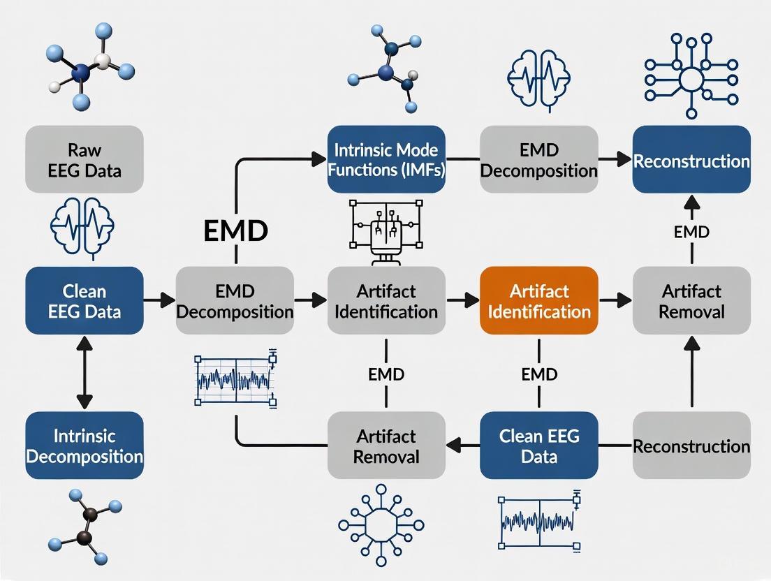
The following workflow diagram illustrates the key stages of this protocol:
Figure 1: EMD-BSS Hybrid Artifact Removal Workflow
Successful implementation of artifact removal pipelines requires both computational tools and validated data. The following table details essential resources for researchers in this field.
Table 2: Essential Research Resources for Ocular Artifact Investigation
| Resource Category | Specific Example / Tool | Function & Application |
|---|---|---|
| Reference Datasets | Semi-simulated EEG/EOG Dataset [1] | Provides contaminated EEG and ground-truth "pure" signals for objective benchmarking of artifact removal algorithms. |
| Decomposition Algorithms | EMD Toolbox; Blind Source Separation (BSS) algorithms (e.g., AMICA, Infomax ICA) [1] | Core computational methods for decomposing signals into constituent modes or sources for artifact isolation. |
| Performance Metrics | Spearman Correlation Coefficient (SCC), Root Mean Square Error (RMSE), Signal-to-Artifact Ratio (SAR) [1] | Quantitative measures to evaluate the performance of an artifact removal technique in terms of fidelity and artifact suppression. |
| Machine Learning Classifiers | Artificial Neural Network (ANN) with Scalp Topography feature [8] | For automated detection and classification of artifact-contaminated epochs within EEG data. |
| Deep Learning Frameworks | AnEEG (LSTM-based GAN) [5] | Advanced, data-driven models for end-to-end learning and generation of artifact-free EEG signals from contaminated inputs. |
The critical challenge of ocular artifacts in EEG analysis demands sophisticated and carefully validated solutions. While techniques like the EMD-BSS hybrid approach offer robust, data-driven pathways for artifact removal, the choice of methodology must be aligned with the specific research goals, EEG setup, and required fidelity of neural signal preservation. The protocols and resources provided herein are designed to equip researchers and drug development professionals with the practical knowledge to enhance the quality and reliability of their EEG data, thereby strengthening the conclusions drawn from neural signal analysis in both clinical and research settings.
Fundamental Principles of Empirical Mode Decomposition (EMD)
Core Principles and Mathematical Foundation
Empirical Mode Decomposition (EMD) is an adaptive, data-driven technique designed for analyzing nonlinear and non-stationary signals. Unlike traditional methods that rely on predetermined basis functions, EMD adapts to the signal's inherent characteristics, making it particularly suitable for complex biological signals like electroencephalogram (EEG) which often contain ocular artifacts [9].
The fundamental objective of EMD is to decompose a given input signal ( I(n) ) into a series of oscillatory components, known as Intrinsic Mode Functions (IMFs), and a residual component. This decomposition is represented as [9]: [ I(n) = \sum{m=1}^{M} IMF{m}(n) + Res{M}(n) ] Here, ( IMF{m}(n) ) denotes the ( m )-th IMF, and ( Res_{M}(n) ) is the final residue after extracting ( M ) IMFs. The residue represents the signal's overall trend, while the IMFs capture oscillatory modes from high to low frequencies.
An IMF must satisfy two key conditions to ensure meaningful instantaneous frequency analysis:
- The number of extrema (maxima and minima) and the number of zero-crossings must either be equal or differ at most by one.
- The mean value of the envelope defined by the local maxima and the envelope defined by the local minima is zero at any point.
The EMD algorithm, often termed a sifting process, iteratively extracts IMFs through the following steps [9]:
- Identify all local extrema (maxima and minima) of the input signal ( I(n) ).
- Construct the upper envelope ( e{\text{max}}(n) ) by connecting all local maxima, and the lower envelope ( e{\text{min}}(n) ) by connecting all local minima, typically using cubic spline interpolation.
- Compute the mean envelope ( m(n) = [e{\text{max}}(n) + e{\text{min}}(n)] / 2 ).
- Subtract the mean envelope from the signal to obtain a proto-IMF: ( h(n) = I(n) - m(n) ).
- Check if ( h(n) ) satisfies the IMF conditions. If not, repeat steps 1-4 using ( h(n) ) as the new input signal until the conditions are met.
- Once the conditions are met, designate the resulting ( h(n) ) as an IMF component ( IMF_{m}(n) ).
- Subtract this IMF from the original signal to obtain the residue: ( r(n) = I(n) - IMF_{m}(n) ).
- Repeat the entire process on the residual ( r(n) ) to extract the next IMF. The process stops when the residue becomes a monotonic function from which no more IMFs can be extracted.
Addressing the Mode-Mixing Problem with Ensemble EMD
A significant challenge in the standard EMD algorithm is mode mixing, where oscillations of dramatically different scales are assigned to a single IMF, or similar-scale oscillations are split across multiple IMFs. This phenomenon can obscure the physical meaning of the extracted components and is often triggered by intermittent signals or the presence of noise [10].
Ensemble Empirical Mode Decomposition (EEMD) was developed to mitigate mode mixing by leveraging the statistical properties of noise. The core idea is to decompose the original signal multiple times, each time with added white noise of finite amplitude. The white noise provides a uniform reference scale distribution, ensuring that the signal of interest is projected onto a uniform set of reference scales in the noise background. The true IMFs are then defined as the mean of the corresponding components from the ensemble of trials, effectively canceling out the added noise [10].
The EEMD procedure is as follows [10]:
- Add White Noise: Generate a new noisy signal ( xi(t) = x(t) + wi(t) ), where ( w_i(t) ) is a white noise series of a predetermined amplitude, and ( i ) is the trial number.
- Decompose: Apply the standard EMD algorithm to ( x_i(t) ), decomposing it into a set of IMFs.
- Ensemble Averaging: Repeat steps 1 and 2 ( N ) times, each time with a different, independently generated white noise series. The final, true IMF is obtained by averaging the corresponding IMFs from all ensemble trials: [ IMF{m}^{\text{(final)}}(t) = \frac{1}{N} \sum{i=1}^{N} IMF_{m}^{(i)}(t) ]
A critical aspect of EEMD is the selection of two key parameters: the ensemble number ( N ) and the amplitude of the added white noise. A well-demonstrated statistical rule guides this selection [10]: [ \epsilonN = \frac{\epsilon}{\sqrt{N}} ] where ( \epsilon ) is the amplitude of the added white noise and ( \epsilonN ) is the standard deviation of the final error. This relationship indicates that the effect of the added noise decreases as the ensemble size increases. Prior studies have found that parameter settings with an ensemble number of 100 and a noise amplitude of 0.2 times the standard deviation of the original signal typically yield satisfactory results [10].
EMD for Ocular Artifact Removal in EEG
Ocular artifacts, primarily caused by eye blinks and movements, present a major challenge in EEG analysis. These artifacts manifest as low-frequency, high-amplitude signals that can obscure underlying neural activity. EMD and its variants offer a powerful, data-driven solution for cleaning single-channel EEG recordings, where traditional multi-channel techniques like Independent Component Analysis (ICA) are less effective [2].
The general workflow for EMD-based ocular artifact removal is as follows:
- Decomposition: The contaminated EEG signal ( x(t) ) is decomposed into a set of IMFs using the EMD or EEMD algorithm.
- Identification: The IMFs correlated with the ocular artifact are identified. This step often employs statistical metrics such as Kurtosis (KS), Dispersion Entropy (DisEn), and Power Spectral Density (PSD). Artifactual components typically exhibit high kurtosis (indicating peakedness) and dominant power in the low-frequency range (e.g., 0.5-12 Hz) characteristic of eye blinks [2].
- Removal/Filtering: The identified artifact-laden IMFs are processed to remove the artifactual content. This can be done by:
- Complete Removal: Setting the entire artifactual IMF to zero.
- Thresholding: Applying a filtering technique, such as the Generalized Moreau Envelope Total Variation (GMETV) filter, to suppress only the artifact segments within the IMF while preserving neural information [2].
- Reconstruction: The cleaned signal ( \hat{x}(t) ) is reconstructed by summing the remaining processed and unprocessed IMFs along with the final residue.
Table 1: Quantitative Metrics for Evaluating EMD-based Artifact Removal
| Metric | Formula | Interpretation in Artifact Removal Context |
|---|---|---|
| Root Relative Mean Squared Error (RRMSE) [11] | ( RRMSE = \sqrt{\frac{\sum{n=1}^{N} (x{\text{clean}}(n) - x{\text{denoised}}(n))^2}{\sum{n=1}^{N} x_{\text{clean}}(n)^2}} ) | Measures the overall difference between the clean and denoised signal. Lower values indicate better artifact removal and signal preservation. |
| Correlation Coefficient (CC) [11] | ( CC = \frac{\text{cov}(x{\text{clean}}, x{\text{denoised}})}{\sigma{x{\text{clean}}} \sigma{x{\text{denoised}}}} ) | Quantifies the linear relationship between the clean and denoised signal. Values closer to 1 indicate better preservation of the original signal's structure. |
| Signal-to-Artifact Ratio (SAR) [2] | ( SAR = 10 \log_{10}\left(\frac{\text{Power of clean part}}{\text{Power of artifact}}\right) ) | Measures the improvement in signal quality after artifact removal. Higher values indicate more effective artifact suppression. |
Experimental Protocol: Ocular Artifact Removal Using EEMD
This protocol provides a detailed methodology for removing ocular artifacts from a single-channel EEG recording using the EEMD technique.
Materials and Reagents
- EEG Data: Raw single-channel EEG recording suspected to contain ocular artifacts.
- Computing Environment: Software with EMD/EEMD implementation (e.g., MATLAB, Python with
PyEMDorEMDpackage). - Ground Truth (Optional): Simultaneously recorded EOG signal or a clean segment of EEG for validation.
Procedure
Data Preprocessing:
- Import the raw EEG signal ( x_{\text{raw}}(t) ).
- Apply a band-pass filter (e.g., 0.5-45 Hz) to remove DC offset and high-frequency noise, if necessary. Let the preprocessed signal be ( x(t) ).
Ensemble EMD Decomposition:
- Set the EEMD parameters: ensemble number ( N = 100 ) and noise amplitude ( \epsilon = 0.2 \times \text{std}(x(t)) ) (standard deviation of the signal) [10].
- For ( i = 1 ) to ( N ): a. Generate a white noise series ( wi(t) ) with amplitude ( \epsilon ). b. Form a noisy signal: ( xi(t) = x(t) + wi(t) ). c. Decompose ( xi(t) ) using standard EMD to obtain a set of IMFs ( [IMF1^{(i)}, IMF2^{(i)}, ..., IMF_M^{(i)}] ).
- For each IMF mode ( m ), compute the ensemble average: ( IMFm(t) = \frac{1}{N} \sum{i=1}^{N} IMF_m^{(i)}(t) ).
- The final decomposition of ( x(t) ) is the set ( {IMF1(t), IMF2(t), ..., IMFM(t), ResM(t)} ).
Artifact Component Identification:
- For each IMF ( IMF_m(t) ), calculate its statistical features:
- Kurtosis (KS): Compute the kurtosis of the IMF. IMFs with exceptionally high kurtosis are likely contaminated by spike-like artifacts such as eye blinks [2].
- Power Spectral Density (PSD): Estimate the PSD of the IMF. IMFs whose power is concentrated in the low-frequency band (0.5-12 Hz) are strong candidates for containing ocular artifacts [2].
- Based on a pre-defined threshold (e.g., kurtosis > 3, or dominant frequency < 4 Hz), identify the IMF indices ( \mathcal{A} ) that correspond to the ocular artifact.
- For each IMF ( IMF_m(t) ), calculate its statistical features:
Artifact Removal and Signal Reconstruction:
- For each IMF index ( m ) in the artifact set ( \mathcal{A} ), apply the GMETV filter to suppress the artifact:
- ( IMFm^{\text{clean}}(t) = \text{GMETF-Filter}(IMFm(t)) ) [2].
- For all other IMFs ( m \notin \mathcal{A} ), retain the original component: ( IMFm^{\text{clean}}(t) = IMFm(t) ).
- Reconstruct the denoised EEG signal: [ x{\text{denoised}}(t) = \sum{m=1}^{M} IMFm^{\text{clean}}(t) + ResM(t) ]
- For each IMF index ( m ) in the artifact set ( \mathcal{A} ), apply the GMETV filter to suppress the artifact:
Validation and Performance Assessment:
- If a ground truth clean signal ( x_{\text{clean}}(t) ) is available, compute the performance metrics from Table 1 (RRMSE, CC, SAR).
- Visually inspect the denoised signal ( x_{\text{denoised}}(t) ) and compare it with the original contaminated signal ( x(t) ) to confirm artifact removal.
Visualization of the EEMD-based Artifact Removal Workflow
The Scientist's Toolkit: Key Reagents and Computational Tools
Table 2: Essential Materials and Computational Tools for EMD Research
| Item | Type | Function/Application |
|---|---|---|
| Single-Channel EEG Data | Data | The primary input signal contaminated with ocular artifacts for analysis and cleaning [2]. |
| White Noise Generator | Algorithm | Produces the finite-amplitude noise series required for the EEMD ensemble process to counteract mode mixing [10]. |
| Cubic Spline Interpolation | Algorithm | The standard method for constructing the upper and lower envelopes during the EMD sifting process by connecting local extrema [9]. |
| Kurtosis (KS) | Statistical Metric | A measure of the "tailedness" of a signal distribution; used to identify spike-like artifacts in IMFs [2]. |
| Power Spectral Density (PSD) | Signal Processing Metric | Estimates the signal's power distribution across frequencies; used to identify IMFs dominated by low-frequency ocular artifacts [2]. |
| Generalized Moreau Envelope Total Variation (GMETV) Filter | Filtering Algorithm | A specialized filter applied to artifact-laden IMFs to suppress artifacts while preserving the underlying neural signal morphology [2]. |
| Ground Truth EOG/EEG | Validation Data | A simultaneously recorded EOG signal or a clean EEG segment used to validate the performance of the artifact removal algorithm [2]. |
Characteristics and Impact of Ocular Artifacts on Neural Data
Electroencephalogram (EEG) is a fundamental non-invasive tool for measuring electrical brain activity, widely used in neuroscience research, clinical diagnosis, and brain-computer interfaces. However, the recorded EEG signals are frequently contaminated by various artifacts, among which ocular artifacts present a particularly significant challenge. These artifacts, generated by eye movements and blinks, can severely obscure neural signals of interest and lead to misinterpretation in both research and clinical settings [1] [12].
Ocular artifacts originate from the corneo-retinal potential, which creates an electric dipole across the eye. This dipole moves with gaze direction, generating electrical potentials that spread across the scalp and contaminate EEG recordings [12]. The impact is especially problematic because the spectral characteristics of ocular artifacts overlap substantially with fundamental neural rhythms, particularly in the delta and theta frequency bands [2] [12]. This spectral overlap complicates the use of simple filtering techniques, as they would remove crucial neural information along with the artifacts.
Within the broader context of empirical mode decomposition (EMD) research for ocular artifact removal, this application note provides a comprehensive overview of the characteristics of ocular artifacts, quantitative performance comparisons of contemporary removal techniques, detailed experimental protocols, and essential research tools to support researchers in implementing these methods effectively.
Characteristics and Challenges of Ocular Artifacts
Physiological Origins and Types
Ocular artifacts primarily manifest in two distinct forms with different properties:
Saccadic Artifacts: Result from rapid eye movements between fixation points. These appear as changes in signal offset with amplitudes roughly proportional to saccade size, exhibiting highest spectral power in the 4-20 Hz range. Their spatial distribution varies with gaze direction, affecting primarily frontal and fronto-temporal sensors [12].
Blink Artifacts: Caused by eyelid movement over the cornea during blinking. These manifest as sharp, high-amplitude spikes lasting hundreds of milliseconds, with spectral content concentrated below 5 Hz. Unlike saccades, blink artifacts affect frontal sensors bilaterally with consistent spatial patterns [12].
Impact on Neural Data Analysis
The presence of ocular artifacts significantly compromises EEG data quality and interpretation:
Amplitude Distortion: Ocular artifacts typically exhibit amplitudes 5-10 times greater than background neural activity, potentially obscuring event-related potentials and other neural phenomena [2].
Spectral Contamination: The overlapping frequency content between ocular artifacts (0.5-20 Hz) and fundamental EEG rhythms (delta: 0.5-4 Hz, theta: 4-8 Hz, alpha: 8-13 Hz) makes complete separation challenging [2] [12].
Topographical Spread: Ocular artifacts volume-conduct through cerebrospinal fluid, skull, and scalp, affecting widespread electrode sites with maximal impact on frontal regions [12].
Quantitative Performance Comparison of Ocular Artifact Removal Methods
Table 1: Performance Metrics of Contemporary Ocular Artifact Removal Techniques
| Method | Core Approach | Signal Domain | SCC | RMSE | SAR | Key Advantages |
|---|---|---|---|---|---|---|
| EMD-BSS [1] | Empirical Mode Decomposition + Blind Source Separation | Multi-channel | 0.95 | 9.51 | 1.92 | Superior artifact rejection efficacy |
| EMD-AMICA [1] | EMD + Adaptive Mixture ICA | Multi-channel | 0.95 | 9.51 | 1.92 | Optimal performance in hybrid methodology |
| FF-EWT+GMETV [2] | Fixed Frequency EWT + Generalized Moreau Envelope Filter | Single-channel | N/R | Low RRMSE | Improved | Excellent for portable SCL EEG systems |
| AOAR [13] | NMF + EMD + Fractal Dimension | Multi-channel | High | Low | High SNR | Superior for ADHD classification applications |
| EICA [14] | Ensemble EMD + ICA | Multi-channel | High | Low | High SNR | Effectively eliminates blink artifacts with minimal error |
| SVM-VMD-SOBI [15] | Support Vector Machine + VMD + SOBI | Single-channel | N/R | Minimal | N/R | Minimizes signal distortion in OSAS patients |
| AnEEG [5] | LSTM-based GAN | Multi-channel | High | Low | High | Preserves temporal dependencies in neural activity |
SCC: Spearman Correlation Coefficient; RMSE: Root Mean Square Error; SAR: Signal-to-Artifact Ratio; SNR: Signal-to-Noise Ratio; N/R: Not Reported
Table 2: Application Context and Limitations of Ocular Artifact Removal Methods
| Method | Best-Suited Applications | Computational Complexity | Key Limitations |
|---|---|---|---|
| EMD-BSS [1] | Research settings requiring high-fidelity artifact removal | Moderate to High | May require manual component identification |
| FF-EWT+GMETV [2] | Portable healthcare monitoring devices | Moderate | Optimized for specific artifact types |
| AOAR [13] | Clinical populations (e.g., ADHD) | Moderate | Requires normalization for non-negativity |
| EICA [14] | Multichannel research datasets | High | EEMD computation intensive |
| SVM-VMD-SOBI [15] | Sleep studies (OSAS patients) | High | Requires pre-trained SVM classifier |
| AnEEG [5] | Large-scale research datasets | Very High | Requires extensive training data |
Detailed Experimental Protocols
Comprehensive EMD-BSS Protocol for Multi-channel EEG Data
The EMD-BSS hybrid methodology combines the adaptive decomposition capability of Empirical Mode Decomposition with the source separation power of Blind Source Separation algorithms [1].
Table 3: Research Reagent Solutions for EMD-BSS Protocol
| Research Reagent | Function/Application | Implementation Notes |
|---|---|---|
| EEG Recording System | Signal acquisition | 16+ channels recommended for optimal BSS performance |
| EOG Reference Electrodes | Artifact reference recording | Placed at supraorbital and canthal positions |
| EMD Algorithm | Signal decomposition into IMFs | Ensures proper stopping criteria to prevent over-decomposition |
| BSS Algorithms (AMICA, SOBI, etc.) | Source separation | AMICA often performs best for ocular artifacts [1] |
| Fractal Dimension Analysis | Automatic artifact component identification | Alternative: kurtosis, entropy, or sample entropy metrics |
| Signal Reconstruction Toolbox | Component removal and signal reconstruction | Custom MATLAB/Python scripts for inversion process |
Step-by-Step Procedure:
Data Acquisition and Preprocessing
- Record EEG data using standard international 10-20 system placement with additional EOG electrodes for reference.
- Apply band-pass filtering (0.5-45 Hz) to remove extreme frequency components while preserving neural signals.
- Segment data into epochs appropriate for your experimental paradigm.
EMD Decomposition
- Apply EMD to each EEG channel separately to decompose signals into Intrinsic Mode Functions (IMFs).
- For each channel x(t): x(t) = Σ IMFᵢ(t) + rₙ(t), where IMFᵢ represents the i-th mode and rₙ the residue.
- Validate IMF properties: (1) Number of extrema and zero-crossings differ by at most one; (2) Mean of upper and lower envelopes is zero.
Blind Source Separation
- Combine corresponding IMFs across channels to create multi-channel datasets for each mode level.
- Apply BSS algorithm (AMICA recommended) to separate sources from each IMF level.
- For SOBI alternative: use joint approximate diagonalization of covariance matrices at multiple time lags.
Artifact Component Identification
- Calculate artifact-related features for each component: fractal dimension, kurtosis, entropy.
- Establish threshold criteria for automatic identification of ocular artifact components.
- Validate identification against EOG reference channels if available.
Signal Reconstruction
- Remove components identified as ocular artifacts through component zeroing or regression-based subtraction.
- Reconstruct artifact-free IMFs for each channel.
- Apply inverse EMD to reconstruct clean EEG signals.
Diagram 1: EMD-BSS artifact removal workflow
Advanced Single-Channel Protocol Using SVM-VMD-SOBI
For single-channel EEG systems commonly used in portable and clinical applications, this protocol combines machine learning detection with sophisticated decomposition techniques [15].
Step-by-Step Procedure:
Artifact Contamination Detection
- Extract features from EEG segments: amplitude, frequency distribution, entropy, and temporal characteristics.
- Apply pre-trained SVM classifier with Gaussian radial basis function kernel to identify artifact-contaminated segments.
- Use genetic algorithm optimization for SVM parameter tuning if sufficient training data available.
Variational Mode Decomposition
- Optimize VMD parameters (number of modes, bandwidth constraint) using genetic algorithm.
- Decompose identified artifact segments into variational mode functions (VMFs): x(t) = Σ VMFₖ(t).
- Ensure mode bandwidth limitations to prevent spectral overlap.
Second-Order Blind Identification
- Apply SOBI to VMFs to separate underlying sources.
- Compute covariance matrices at multiple time lags for joint approximate diagonalization.
- Extract independent components from the VMF representations.
Approximate Entropy Thresholding
- Calculate approximate entropy for each component: ApEn(m,r,N) where m is pattern length, r is tolerance, N is data length.
- Establish entropy threshold based on clean EEG baseline measurements.
- Remove components exceeding entropy threshold (indicating high irregularity characteristic of artifacts).
Signal Reconstruction
- Apply inverse SOBI transformation to retained components.
- Reconstruct artifact-corrected segment using inverse VMD.
- Merge corrected segments with uncontaminated EEG portions.
Diagram 2: Single-channel artifact removal process
The Scientist's Toolkit
Table 4: Essential Research Reagents and Computational Tools
| Tool Category | Specific Tools/Software | Research Application | Implementation Considerations |
|---|---|---|---|
| Decomposition Algorithms | EMD, EEMD, VMD, EWT | Signal separation into components | EEMD addresses mode mixing in standard EMD [14] |
| Blind Source Separation | ICA, SOBI, AMICA, CCA | Source separation from mixed signals | AMICA often outperforms standard ICA for ocular artifacts [1] [12] |
| Machine Learning Classifiers | SVM, Random Forest, CNN | Automated artifact identification | SVM effective for segment identification with limited training data [15] |
| Deep Learning Frameworks | LSTM, GAN, Transformer Networks | End-to-end artifact removal | AnEEG (LSTM-GAN) shows promise for temporal dependency preservation [5] |
| Signal Processing Platforms | EEGLAB, FieldTrip, MNE-Python | Comprehensive processing pipelines | EEGLAB includes ICA implementation and component visualization tools |
| Performance Metrics | SCC, RMSE, SAR, SNR | Method validation and comparison | Multi-metric assessment provides comprehensive performance evaluation [1] [2] |
Ocular artifacts present significant challenges in neural data analysis due to their high amplitude, spectral overlap with neural signals, and spatial distribution across the scalp. Contemporary removal methodologies have evolved from simple regression and filtering approaches to sophisticated hybrid methods that combine the strengths of multiple techniques. The EMD-based approaches, particularly when integrated with BSS algorithms, provide powerful frameworks for addressing these contaminants while preserving neural information essential for accurate data interpretation.
For researchers implementing these methods, selection should be guided by specific application requirements: multi-channel research settings benefit from EMD-BSS hybrids, while single-channel applications may require SVM-VMD-SOBI approaches. Recent advances in deep learning, particularly LSTM-GAN architectures, show promising directions for future development with potential for improved preservation of temporal dynamics in neural signals. Through careful implementation of these protocols and consideration of the quantitative performance metrics provided, researchers can significantly enhance EEG data quality for more accurate neural analysis.
Advantages of EMD for Non-Stationary Biological Signals
Empirical Mode Decomposition (EMD) has emerged as a transformative methodology for analyzing non-stationary biological signals, particularly in ocular artifact removal from electroencephalogram (EEG) data. Unlike traditional signal processing techniques that rely on predefined basis functions, EMD adaptively decomposes complex, non-stationary signals into their intrinsic oscillatory components, known as Intrinsic Mode Functions (IMFs). This data-driven approach enables superior handling of nonlinear, non-stationary signals commonly encountered in physiological recordings. Recent advancements, including hybrid methodologies combining EMD with Blind Source Separation (BSS) techniques, have demonstrated significant performance improvements in artifact removal while preserving underlying neural information. This application note comprehensively outlines the theoretical advantages, quantitative performance metrics, and detailed experimental protocols for implementing EMD-based approaches in biomedical signal processing, with particular emphasis on ocular artifact removal for clinical and research applications.
Biological signals, including electroencephalography (EEG), electrocardiography (ECG), and electromyography (EMG), are inherently non-stationary, meaning their statistical properties change over time. These signals typically exhibit nonlinear dynamics and complex frequency modulations that challenge conventional signal processing techniques like Fourier analysis and wavelet transforms, which assume signal stationarity or require predefined basis functions [16] [17].
Empirical Mode Decomposition (EMD), introduced by Huang et al. in 1998, represents a fundamentally different approach—it is fully data-driven and adaptive. The algorithm iteratively decomposes any complex signal into a finite set of oscillatory components called Intrinsic Mode Functions (IMFs) through a sifting process that relies solely on the signal's local extrema [17]. This intrinsic adaptability makes EMD particularly suitable for processing physiological signals where prior knowledge of signal characteristics may be limited or inadequate.
In the specific context of ocular artifact removal, EMD offers distinct advantages. Ocular artifacts originating from eye blinks and movements manifest as high-amplitude, low-frequency distortions in EEG recordings, often overlapping with the frequency range of neural signals of interest. Traditional filtering approaches often remove neural information along with artifacts, whereas EMD enables more selective isolation and removal of artifact components while preserving cerebral activity [1] [2].
Theoretical Advantages of EMD for Biological Signal Processing
Adaptability to Signal Characteristics
EMD's primary advantage lies in its self-adaptive nature. Unlike Fourier or wavelet transforms that decompose signals using predetermined basis functions, EMD derives its basis functions directly from the signal itself through the sifting process [16]. This allows it to naturally handle nonlinear and non-stationary properties of biological signals without requiring prior assumptions about signal characteristics or parameter tuning.
Localized Time-Frequency Analysis
The EMD method provides inherently localized time-frequency analysis, enabling the identification of transient signal features and localized oscillations. Each extracted IMF represents a specific timescale of oscillation, with the first IMFs capturing fine-scale, high-frequency components and subsequent IMFs representing progressively coarser, lower-frequency oscillations [18]. This multi-resolution analysis capability is particularly valuable for identifying and isolating transient artifacts such as eye blinks that occur intermittently throughout EEG recordings.
Completeness and Orthogonality
The EMD decomposition is theoretically complete, meaning the sum of all IMFs plus the final residue perfectly reconstructs the original signal. Although IMFs are not strictly orthogonal, they approach orthogonality in practice, minimizing energy leakage between components and enabling effective separation of signal and artifact components [19].
Handling Multidimensional Data
Recent extensions of EMD, such as the Multidimensional and Multivariate Fast Iterative Filtering (MdMvFIF) technique, have expanded its applicability to complex multidimensional and multivariate biological signals [18]. These advancements allow simultaneous processing of signals that vary across both space and time, making EMD suitable for modern high-density EEG arrays and other multichannel physiological recording systems.
Quantitative Performance Analysis
Recent studies have demonstrated the superior performance of EMD-based approaches for ocular artifact removal compared to conventional techniques. The tables below summarize key quantitative findings from comparative studies.
Table 1: Performance Metrics of EMD-BSS Hybrid Method for Ocular Artifact Removal
| Algorithm | Spearman Correlation Coefficient (SCC) | Root Mean Square Error (RMSE) | Euclidean Distance (ED) | Signal-to-Artifact Ratio (SAR) |
|---|---|---|---|---|
| EMD-AMICA | 0.95 | 9.51 | 736.7 | 1.92 |
| EMD-SOBI | 0.91 | 10.82 | 821.4 | 1.65 |
| EMD-FastICA | 0.89 | 11.75 | 894.2 | 1.43 |
| Standard BSS | 0.76-0.84 | 12.94-15.63 | 953.1-1120.5 | 0.95-1.27 |
Data sourced from [1] demonstrating performance metrics averaged across 54 datasets.
Table 2: Clinical Application Accuracy of EMD Across Medical Domains
| Application Domain | Physiological Signal | Reported Accuracy | Key Advantage |
|---|---|---|---|
| Neurology | EEG | Up to 98% detection accuracy for epileptic seizures | Enhanced sensitivity for transient events |
| Cardiology | ECG | Up to 98% for detecting cardiac abnormalities | Superior to Fourier and wavelet transforms |
| Respiratory Medicine | Respiratory patterns | 20% reduction in false-positive rates | Improved computational efficiency |
Data compiled from clinical validation studies [20].
Experimental Protocols
Protocol 1: Standard EMD for Single-Channel Ocular Artifact Removal
Purpose: Remove ocular artifacts from single-channel EEG recordings using standard EMD decomposition.
Materials and Reagents:
- Raw EEG data (continuous recording)
- Computing environment with EMD implementation (MATLAB, Python, or SAS/IML)
- Cubic spline interpolation algorithm
Procedure:
Signal Preprocessing:
- Import raw EEG data and apply necessary preprocessing (referencing, baseline correction)
- If required, resample data to appropriate frequency (typically 250-500 Hz)
- Detrend the signal by removing linear or slow polynomial trends
EMD Decomposition:
- Identify all local extrema (maxima and minima) in the input signal
- Interpolate between maxima to create upper envelope, and between minima to create lower envelope using cubic spline interpolation
- Compute the mean of the upper and lower envelopes (m1)
- Subtract the mean from the original signal to obtain the first component (h1): h1 = x(t) - m1
- Check if h1 satisfies IMF conditions (number of extrema and zero-crossings differs by at most one; mean of envelopes is zero)
- If IMF conditions are not met, repeat the sifting process on h1 (typically 4-10 iterations)
- Once IMF conditions are satisfied, designate the component as IMF1
- Subtract IMF1 from the original signal to obtain the residue (r1 = x(t) - IMF1)
- Repeat the process on the residual until the final residue is monotonic or contains at most one extremum
Ocular Artifact Identification:
- Identify IMFs containing ocular artifacts typically IMFs 1-3 for eye blinks (0.5-4 Hz range)
- Apply additional validation using kurtosis, power spectral density, or correlation with EOG reference channel if available
Signal Reconstruction:
- Reconstruct cleaned EEG signal by summing all IMFs excluding those identified as artifact components
- Verify reconstruction quality by ensuring signal continuity and absence of discontinuities
Validation:
- Compute correlation between cleaned signal and artifact-free baseline recordings
- Calculate Signal-to-Artifact Ratio (SAR) and Root Mean Square Error (RMSE) for performance quantification
- Visually inspect time-domain and frequency-domain representations for residual artifacts
Protocol 2: Hybrid EMD-BSS Methodology for Multi-channel Artifact Removal
Purpose: Implement a hybrid EMD-Blind Source Separation approach for enhanced ocular artifact removal from multi-channel EEG data.
Materials and Reagents:
- Multi-channel EEG data (minimum 8 channels recommended)
- EMD algorithm implementation
- BSS algorithm suite (AMICA, SOBI, FastICA, or similar)
- Semi-simulated EEG dataset with known artifact components for validation [1]
Procedure:
Data Preparation:
- Organize multi-channel EEG data in matrix format (channels × time points)
- Apply bandpass filter (0.5-45 Hz) to remove extreme frequency components
- Select appropriate EEG segment length (typically 30-60 seconds for stable decomposition)
Channel-Wise EMD Decomposition:
- Apply standard EMD (as described in Protocol 1) to each EEG channel independently
- For each channel, obtain full set of IMFs (typically 8-12 components)
- Organize resulting IMFs into a multi-dimensional array (channels × IMFs × time points)
BSS Application:
- Restructure IMF array for BSS processing by concatenating similar-order IMFs across channels
- Apply selected BSS algorithm (AMICA recommended based on performance metrics) to separate neural and artifactual sources
- Identify artifact-related independent components using automated criteria (high low-frequency power, frontal dominance, high kurtosis)
Component Reconstruction and Validation:
- Reconstruct artifact-free IMFs by removing artifact-related components
- Recombine processed IMFs for each channel to obtain cleaned EEG signals
- Apply inverse reconstruction to obtain artifact-free multi-channel EEG data
Validation Metrics:
- Calculate Spearman Correlation Coefficient (SCC) between cleaned signal and pure EEG baseline
- Compute Euclidean Distance (ED) and Root Mean Square Error (RMSE) for quantitative performance assessment
- Compare Signal-to-Artifact Ratio (SAR) before and after processing
- Perform visual inspection of topographical maps and time-frequency representations
Protocol 3: Enhanced EMD with Improved Complete Ensemble EMD (ICEEMDAN)
Purpose: Utilize improved noise-assisted EMD variant to address mode mixing and residual noise issues in standard EMD.
Materials and Reagents:
- Raw EEG data with prominent ocular artifacts
- ICEEMDAN algorithm implementation
- White Gaussian noise generator
- Performance evaluation metrics (SCC, RMSE, ED, SAR)
Procedure:
Ensemble Preparation:
- Generate ensemble of noisy copies by adding white Gaussian noise to original signal
- Typical ensemble size: 100-500 realizations
- Adjust noise amplitude to 0.1-0.2 standard deviation of the original signal
Decomposition Process:
- Apply EMD to each noisy realization in the ensemble
- For each IMF order, compute ensemble average across all realizations
- Obtain final set of IMFs with reduced noise and minimal mode mixing
Artifact Removal:
- Identify artifact-dominated IMFs using correlation analysis with EOG reference or template matching
- Apply threshold-based removal or partial reconstruction excluding artifact components
Signal Reconstruction:
- Sum remaining IMFs to obtain cleaned EEG signal
- Validate using quantitative metrics and visual inspection
Advantages:
- Significantly reduces mode mixing phenomenon common in standard EMD
- Produces components with less residual noise and enhanced physical meaning
- Particularly effective for weak signal extraction in noisy biological recordings [19]
The Scientist's Toolkit: Essential Research Reagents and Materials
Table 3: Essential Research Materials for EMD-Based Ocular Artifact Removal
| Item | Specification | Purpose/Function |
|---|---|---|
| EEG Data Source | Semi-simulated EEG/EOG dataset [1] | Validation and algorithm benchmarking |
| Reference Algorithm | REG-ICA [1] | Performance comparison baseline |
| BSS Algorithms | AMICA, SOBI, FastICA [1] | Hybrid implementation with EMD |
| Computing Environment | MATLAB, Python, or SAS/IML [17] | EMD algorithm implementation |
| Decomposition Methods | EMD, EEMD, CEEMDAN, ICEEMDAN [19] | Signal decomposition variants |
| Validation Metrics | SCC, RMSE, ED, SAR [1] | Quantitative performance assessment |
| Visualization Tools | Time-frequency analysis software | Result interpretation and validation |
Advanced Methodologies and Recent Innovations
Fixed Frequency Empirical Wavelet Transform with EMD
Recent innovations have combined EMD principles with wavelet transforms to create more targeted artifact removal approaches. The Fixed Frequency Empirical Wavelet Transform (FF-EWT) integrated with Generalized Moreau Envelope Total Variation (GMETV) filter represents a significant advancement for single-channel EEG artifact removal [2]. This methodology:
- Automatically identifies contaminated components using kurtosis, dispersion entropy, and power spectral density metrics
- Effectively separates artifact sources while preserving essential low-frequency EEG information
- Demonstrates substantial improvements in Relative Root Mean Square Error (RRMSE) and Correlation Coefficient (CC) on synthetic data
- Shows enhanced Signal-to-Artifact Ratio (SAR) and reduced Mean Absolute Error (MAE) on real EEG recordings
Precise Identification-Based Mode Decomposition
The Precise Identification-based Mode Decomposition (PIMD) method enhances EMD's ability to accurately identify peak and valley points in signals with varying signal-to-noise ratios [21]. This approach:
- Eliminates the need for noise-assisted filtering, preventing loss of critical signal features
- Reduces residual noise in IMFs that can obscure signal characteristics
- Performs rigorous high-low frequency decomposition superior to standard EMD
- Has demonstrated exceptional performance in extracting mechanical fault features, with principles directly applicable to biological signal processing
Empirical Mode Decomposition represents a powerful, adaptive framework for processing non-stationary biological signals, with particular efficacy in ocular artifact removal from EEG recordings. The method's intrinsic ability to handle nonlinear, non-stationary signals without predefined basis functions offers distinct advantages over traditional signal processing techniques.
The integration of EMD with complementary methodologies such as Blind Source Separation has yielded significant performance improvements, with hybrid approaches like EMD-AMICA demonstrating superior artifact rejection efficacy (SCC = 0.95, RMSE = 9.51, SAR = 1.92) compared to individual BSS algorithms [1]. These advancements propel EEG signal purity toward new standards, enabling more accurate neural signal analysis for both clinical and research applications.
Future developments in EMD methodology will likely focus on enhanced mode alignment in multivariate signals, improved boundary effect handling, and deeper integration with machine learning approaches for automated component classification. As EMD continues to evolve, its application in biomedical signal processing promises to expand, offering increasingly sophisticated tools for extracting meaningful information from complex physiological recordings.
Comparison of EMD with Traditional Filtering Approaches
The removal of ocular artifacts from electroencephalography (EEG) signals represents a significant challenge in biomedical signal processing. This application note provides a structured comparison between adaptive, data-driven decomposition techniques, primarily Empirical Mode Decomposition (EMD) and its variants, and traditional filtering approaches for ocular artifact removal. We summarize quantitative performance data, detail experimental protocols for key methodologies, and provide visual workflows to guide researchers in selecting and implementing appropriate denoising strategies. Framed within a broader thesis on EMD-based ocular artifact removal, this document underscores the superior adaptability of EMD-family methods in handling non-stationary biosignals compared to conventional fixed-basis approaches, while also acknowledging the emerging promise of hybrid and deep learning techniques.
Ocular artifacts (OAs), caused by eye blinks and movements, are a predominant source of contamination in electroencephalography (EEG) signals. They are characterized by high amplitude and spectral overlap with the clinically relevant delta and theta brain rhythms, making their removal particularly challenging without distorting underlying neural information [15]. Effective artifact removal is critical in diverse applications, from clinical diagnostics and Brain-Computer Interface (BCI) development to neuropharmacology and cognitive research [4] [22].
The evolution of OA removal techniques has progressed from simple, assumption-heavy traditional filters to more adaptive, data-driven decomposition methods. Traditional filtering approaches, such as regression and fixed-basis transformations, often struggle with the non-stationary and nonlinear nature of EEG signals. In contrast, Empirical Mode Decomposition (EMD) and its advanced variants like Ensemble EMD (EEMD) and Complete EEMD with Adaptive Noise (CEEMDAN) offer a fully data-driven, adaptive framework for signal analysis, which is more suited to the complex characteristics of biological signals [23].
This document systematically compares these methodological families, providing a resource for researchers and scientists engaged in signal preprocessing for drug development and neuroscientific research.
Quantitative Performance Comparison
The following tables summarize the key characteristics and quantitative performance metrics of EMD-based methods against traditional and other modern filtering approaches as reported in recent literature.
Table 1: Comparative Analysis of Signal Processing Techniques for Ocular Artifact Removal.
| Method | Core Principle | Key Advantages | Inherent Limitations |
|---|---|---|---|
| High-Pass Filtering | Applies a fixed frequency cutoff to remove low-frequency artifacts [15]. | Simple to implement, computationally efficient. | Risks removing valuable neural information due to spectral overlap with EEG [15]. |
| Regression-Based Methods | Uses reference EOG signals to estimate and subtract artifact influence from EEG [15]. | Effective with high-quality reference signals. | Requires additional EOG channels, can cause signal distortion due to bidirectional contamination [15]. |
| Blind Source Separation (BSS) | Separates mixed signals into statistically independent sources [24]. | Does not require a reference signal; effective for multi-channel EEG. | Requires multiple channels; performance degrades with low channel counts [4] [15]. |
| Wavelet Transform (WT) | Decomposes signals using pre-defined basis functions into time-frequency components [2] [25]. | Good time-frequency localization. | Performance depends on selection of wavelet base and decomposition level, which is often empirical [15]. |
| Empirical Mode Decomposition (EMD) | Data-driven, adaptive decomposition of non-stationary signals into Intrinsic Mode Functions (IMFs) [23]. | Does not require pre-defined basis; self-adaptive to signal content. | Prone to mode mixing and noise sensitivity [23]. |
| Variational Mode Decomposition (VMD) | Non-recursive decomposition that solves a constrained optimization problem to obtain modes [26]. | Resists mode mixing; more robust to noise than EMD. | Requires careful parameter selection (e.g., number of modes, bandwidth) [26]. |
Table 2: Reported Performance Metrics of Advanced Decomposition and Hybrid Methods.
| Methodology | Application Context | Reported Performance Metrics | Citation |
|---|---|---|---|
| VMD + Random Forest | Power Quality Disturbance (PQD) Classification | Classification Accuracy: 94.6% ± 1.42 (Cross-validation) | [26] |
| FF-EWT + GMETV Filter | EOG Artifact Removal from Single-Channel EEG | Lower RRMSE, Higher CC and SAR on synthetic and real data. | [2] |
| VMD-BSS | Ocular Artifact Removal from Multi-channel EEG | Strong Correlation Coefficient: 0.82; Minimal Euclidean Distance: 704.04 | [24] |
| SVM + GA-VMD + SOBI | Ocular Artifact Removal from Single-Channel EEG | Effectively mitigated ocular artifacts while minimizing EEG signal distortion in OSAS patients. | [15] |
| EMD-based Dictionary | Patient-Specific Seizure Detection | Accuracy: 88.2%, Sensitivity: 90.3%, Specificity: 88.1% | [25] |
| Fingerprint + ARCI + SPHARA | Dry EEG Denoising | Improved Grand Average SD from 9.76 μV to 6.72 μV; Improved SNR. | [27] |
Detailed Experimental Protocols
Protocol 1: Ocular Artifact Removal using SVM with GA-VMD and SOBI
This protocol details a sophisticated dual-decomposition and dual-recognition strategy for single-channel EEG, integrating machine learning and signal decomposition for targeted artifact removal [15].
A. Signal Preprocessing and Artifact Detection
- Data Acquisition: Acquire single-channel EEG data according to the experimental paradigm.
- Preprocessing: Apply a band-pass filter (e.g., 0.5-40 Hz) and a notch filter (50/60 Hz) to remove line noise.
- Segmentation: Segment the continuous EEG into epochs.
- Artifact Identification: Feed epochs into a pre-trained Support Vector Machine (SVM) classifier to identify segments contaminated with ocular artifacts. The SVM is trained on features derived from historical data to distinguish between clean and artifact-laden epochs.
B. Genetic Algorithm-Optimized VMD
- Parameter Optimization: Use a Genetic Algorithm (GA) to optimize key VMD parameters, primarily the number of modes
Kand the bandwidth parameterα. The fitness function is typically designed to maximize sparsity or separation quality. - Signal Decomposition: Apply the optimized VMD to the artifact-contaminated segments identified by the SVM. This decomposes the signal into
Kband-limited Variational Mode Functions (VMFs).
- Parameter Optimization: Use a Genetic Algorithm (GA) to optimize key VMD parameters, primarily the number of modes
C. Second-Order Blind Identification (SOBI) and Component Removal
- Source Separation: Apply the SOBI algorithm to the set of VMFs obtained from the previous step. SOBI further decomposes them into underlying sources by jointly diagonalizing a set of covariance matrices at different time lags.
- Feature Calculation: Calculate the approximate entropy of each component resulting from the SOBI decomposition.
- Thresholding: Set an approximate entropy threshold to identify components correlated with ocular artifacts. Components with entropy values exceeding the threshold are considered artifactual.
- Component Removal: Discard the artifact-laden components.
D. Signal Reconstruction
- Apply the inverse SOBI transformation to the remaining components.
- Apply the inverse VMD process to reconstruct the "clean" EEG signal from the purified VMFs.
- Reintegrate the cleaned segments with the epochs originally classified as clean by the SVM.
Protocol 2: Hybrid VMD-BSS for Multi-Channel EEG
This protocol describes a hybrid approach combining Variational Mode Decomposition with Blind Source Separation for effective artifact removal in multi-channel EEG setups [24].
A. Signal Preprocessing
- Acquire multi-channel EEG data according to the international 10-20 system.
- Preprocess the data: apply a notch filter (50/60 Hz) and optionally a band-pass filter.
B. Variational Mode Decomposition
- For each EEG channel, apply VMD to decompose the signal into a pre-defined number of Intrinsic Mode Functions (IMFs). The number of modes
Kis a critical parameter that may be set empirically or via an optimization procedure. - The full dataset now consists of the original channels, each represented by a set of IMFs.
- For each EEG channel, apply VMD to decompose the signal into a pre-defined number of Intrinsic Mode Functions (IMFs). The number of modes
C. Blind Source Separation
- Aggregate the IMFs from all channels into a new multi-dimensional input.
- Apply a BSS algorithm (e.g., Independent Component Analysis - ICA) to this aggregated data to separate it into statistically independent components.
D. Artifact Component Identification and Removal
- Identify components corresponding to ocular artifacts. This can be achieved through:
- Visual inspection of component topographies and time courses.
- Automated algorithms based on features like kurtosis, power spectral density, or correlation with EOG reference signals if available [2].
- Remove the components identified as artifacts.
- Identify components corresponding to ocular artifacts. This can be achieved through:
E. Signal Reconstruction
- Apply the inverse BSS transformation to the remaining components to reconstruct the IMF space.
- For each channel, sum the purified IMFs to reconstruct the clean EEG signal for that channel.
The Scientist's Toolkit: Essential Research Reagents & Materials
Table 3: Key Software, Algorithms, and Datasets for EMD and Artifact Removal Research.
| Tool Name / Category | Function / Application | Relevance in Research |
|---|---|---|
| Empirical Mode Decomposition (EMD) | Adaptive, data-driven signal decomposition into Intrinsic Mode Functions (IMFs) [23]. | Core algorithm for non-stationary signal analysis; foundation for many advanced variants. |
| Variational Mode Decomposition (VMD) | Non-recursive, constrained optimization-based mode decomposition [26]. | Mitigates mode-mixing issues of EMD; often delivers superior component separation [26] [24]. |
| Support Vector Machine (SVM) | Supervised machine learning model for classification and regression [15]. | Used for automated identification of artifact-contaminated segments in EEG signals. |
| Genetic Algorithm (GA) | Evolutionary optimization technique for parameter search [15]. | Employed to automatically optimize critical parameters in VMD and other decomposition methods. |
| Second-Order Blind Identification (SOBI) | Blind Source Separation algorithm using second-order statistics [15]. | Effective for separating sources in EEG after initial decomposition, considered robust for this application. |
| Independent Component Analysis (ICA) | Blind Source Separation algorithm that finds statistically independent sources [24]. | Standard method for isolating and removing artifacts from multi-channel EEG data. |
| Public EEG Datasets (e.g., CHB-MIT) | Curated, annotated EEG data for benchmarking [25]. | Essential for validating and comparing the performance of new algorithms against established baselines. |
| Semi-Simulated EEG Datasets | Real EEG data with artificially added, well-characterized artifacts [24]. | Allows for quantitative performance evaluation as the ground truth clean signal is known. |
Implementing EMD-Based Hybrid Methods for Effective Ocular Artifact Removal
The EMD-BSS hybrid methodology represents a significant advancement in the preprocessing of electroencephalogram (EEG) signals, specifically engineered to address the persistent challenge of ocular artifact contamination. This sophisticated framework strategically combines the complementary strengths of Empirical Mode Decomposition (EMD) and Blind Source Separation (BSS) algorithms to achieve superior artifact rejection while preserving underlying neuronal information [1]. Physiological artifacts, particularly those originating from ocular activity such as blinks and eye movements, continue to pose substantial challenges in EEG research due to their high amplitude (typically 100-200 µV) and overlapping frequency characteristics with genuine neural signals [28]. The EMD-BSS approach directly addresses these limitations through a synergistic decomposition process that enhances the identification and isolation of artifactual components from multichannel EEG recordings.
Within the broader context of ocular artifact removal research, this hybrid methodology offers a compelling solution to the critical trade-off between effective artifact removal and the preservation of cerebral activity. Traditional single-technique approaches often suffer from significant limitations: BSS methods alone may struggle with complete artifact separation, while EMD alone can be affected by mode mixing when processing individual channels [1] [29]. The integrated framework substantially improves upon these methods by leveraging EMD's adaptive signal decomposition capabilities to preprocess signals before applying BSS, resulting in enhanced separation efficacy and minimized loss of neurologically meaningful information [1] [24]. This technical breakthrough is particularly valuable for applications requiring high-fidelity EEG signals, including clinical diagnostics, neuromarketing studies, and cognitive neuroscience research where data purity is paramount.
Quantitative Performance Evaluation
The efficacy of the EMD-BSS hybrid methodology has been rigorously validated through comprehensive performance assessment using established quantitative metrics. Evaluation typically employs four key assessment features: the Spearman Correlation Coefficient (SCC), which measures the statistical dependence between the original and cleaned signals; Euclidean Distance (ED), which quantifies the geometric dissimilarity between signal vectors; Root Mean Square Error (RMSE), which assesses the magnitude of reconstruction error; and the Signal-to-Artifact Ratio (SAR), which evaluates the effectiveness of artifact suppression in the reconstructed signal [1]. These metrics collectively provide a multidimensional perspective on algorithm performance, balancing artifact removal efficiency with neural information preservation.
Experimental results demonstrate that the EMD-BSS framework outperforms standalone BSS techniques across multiple performance indicators. As shown in Table 1, the EMD-AMICA algorithm emerges as the optimally performing technique within the hybrid methodology, achieving exceptional scores across all evaluation metrics [1]. The high SCC value (0.95) indicates strong preservation of the original signal characteristics, while the low RMSE (9.51) confirms minimal reconstruction error. The substantial SAR improvement (1.92) reflects enhanced artifact suppression capabilities compared to conventional approaches.
Table 1: Performance Metrics of EMD-BSS Hybrid Algorithms
| Algorithm | Spearman Correlation Coefficient (SCC) | Root Mean Square Error (RMSE) | Euclidean Distance (ED) | Signal-to-Artifact Ratio (SAR) |
|---|---|---|---|---|
| EMD-AMICA | 0.95 | 9.51 | 736.7 | 1.92 |
| EMD-SOBI | 0.94 | 9.85 | 758.2 | 1.88 |
| EMD-EWASO | 0.93 | 10.12 | 781.5 | 1.85 |
| EMD-FASTICA | 0.92 | 10.45 | 799.3 | 1.81 |
| EMD-PCA | 0.91 | 10.87 | 815.6 | 1.78 |
Comparative analysis with other decomposition techniques further validates the effectiveness of the EMD-BSS approach. As illustrated in Table 2, the hybrid methodology demonstrates competitive performance against other contemporary artifact removal frameworks, particularly in balancing artifact rejection with computational efficiency. While Variational Mode Decomposition (VMD) and Discrete Wavelet Transform (DWT) based approaches show respectable performance in specific metrics, the EMD-BSS framework maintains an advantageous balance across all evaluation dimensions [24].
Table 2: Comparative Performance of Different Hybrid Methodologies
| Methodology | Spearman Correlation Coefficient | Euclidean Distance | Computational Efficiency | Artifact Specificity |
|---|---|---|---|---|
| EMD-BSS | 0.82-0.95 | 703-816 | Moderate | Excellent |
| VMD-BSS | 0.82 | 704.04 | Moderate | Very Good |
| DWT-BSS | 0.82 | 703.64 | High | Good |
| EEMD-PCA | 0.79-0.88 | N/A | Low | Good |
Experimental Protocol and Workflow
Data Acquisition and Preparation
The standard experimental protocol for implementing the EMD-BSS hybrid methodology begins with EEG data acquisition using appropriate electrode configurations. The methodology has been validated using a semi-simulated dataset containing EEG recordings from 27 healthy participants (14 males, mean age 28.2±7.5 years; 13 females, mean age 27.1±5.2 years) collected during eyes-closed sessions [1]. Each recording has a 30-second duration with a sampling rate of 200 Hz, acquired using 19 EEG sensors positioned according to the international 10-20 system. Prior to applying the hybrid methodology, preliminary data preprocessing is essential, including the application of a notch filter at 50 Hz to eliminate power line interference and band-pass filtering between 0.5-45 Hz to remove extraneous frequency components [1]. For research focusing specifically on ocular artifacts, it is recommended to use datasets containing marked EOG events or semi-simulated data where clean EEG is artificially contaminated with EOG signals to establish ground truth for validation.
Core EMD-BSS Processing Workflow
The EMD-BSS methodology follows a systematic, multi-stage processing workflow that transforms contaminated EEG inputs into cleaned neural signals. The complete procedure, diagrammed in Figure 1, can be implemented using standard signal processing environments such as MATLAB or Python with appropriate toolboxes.
Figure 1: EMD-BSS Methodology Workflow
Phase 1: EMD Decomposition The first phase involves applying Empirical Mode Decomposition to each channel of the contaminated EEG signal. The EMD algorithm adaptively decomposes the input signal into a series of Intrinsic Mode Functions (IMFs) through an iterative sifting process [1] [29]. Each IMF represents an oscillatory mode embedded in the original signal with its own frequency band, effectively acting as a filter bank tailored to the specific signal characteristics. For ocular artifact removal, typically 6-10 IMFs are generated, with the initial components (IMF1-IMF3) generally containing the highest frequency content and the later components (IMF4+) capturing lower frequency oscillations [1]. The complete set of IMFs forms the basis for subsequent separation processing.
Phase 2: Blind Source Separation The IMF ensemble generated from all EEG channels is forwarded to the BSS processing stage, which applies specialized separation algorithms to isolate independent components. Research has validated five prominent BSS algorithms within the EMD-BSS framework: AMICA (Adaptive Mixture Independent Component Analysis), SOBI (Second Order Blind Identification), EWASO (Efficient Weighted Adaptive Second Order), FASTICA, and PCA (Principal Component Analysis) [1]. These algorithms operate by exploiting statistical properties of the input signals to separate them into independent components (ICs) with minimal mutual information. During this phase, the BSS algorithm generates a separation matrix that transforms the IMF inputs into maximally independent components, some of which represent artifactual sources while others contain neural information.
Phase 3: Component Classification and Reconstruction The final phase involves identifying and removing artifactual components while preserving neural signals. Component classification employs a multi-criteria approach combining temporal, spectral, and spatial features to distinguish ocular artifacts from cerebral activity [1] [30]. As visualized in Figure 2, this decision process integrates multiple特征 to achieve reliable artifact identification.
Figure 2: Component Classification Logic
Following artifact component identification, signal reconstruction proceeds by projecting only the neural components back to the sensor space while excluding those classified as artifactual. This reconstruction process effectively reverses the BSS transformation while omitting the contribution of artifact-related components. The output is a cleaned EEG signal with significantly reduced ocular contamination while preserving the essential neural information necessary for subsequent analysis [1].
The Scientist's Toolkit: Research Reagent Solutions
Successful implementation of the EMD-BSS hybrid methodology requires specific computational tools and analytical resources. Table 3 comprehensively details the essential research reagents and their respective functions within the experimental framework.
Table 3: Essential Research Reagents and Computational Tools
| Research Reagent | Function | Implementation Notes |
|---|---|---|
| Semi-simulated EEG Dataset | Validation and benchmarking | 27 subjects, 19 channels, 30s recordings, 200Hz sampling rate [1] |
| EMD Algorithm | Signal decomposition into IMFs | Adaptive, data-driven decomposition without predefined basis functions [1] [29] |
| BSS Algorithms (AMICA, SOBI, EWASO, FASTICA, PCA) | Source separation and artifact isolation | AMICA demonstrates superior performance for ocular artifacts [1] |
| Performance Metrics (SCC, ED, RMSE, SAR) | Quantitative evaluation of artifact removal | Multi-dimensional assessment of efficacy and signal preservation [1] |
| MATLAB/Python Signal Processing Toolboxes | Implementation environment | EEGLAB, FieldTrip for MATLAB; MNE-Python, PyEEG for Python |
| Component Classification Criteria | Artifact identification | Temporal, spectral, and spatial features combined for decision logic [30] |
Technical Considerations and Implementation Guidelines
Parameter Optimization
Successful implementation of the EMD-BSS methodology requires careful attention to parameter configuration to balance computational efficiency with artifact rejection performance. For the EMD phase, critical parameters include the stopping criterion for the sifting process (typically between 0.05-0.20) and the maximum number of IMFs to extract (usually 6-10 for EEG signals) [1]. Within the BSS phase, algorithm-specific parameters must be optimized: for AMICA, the number of mixture models and maximum iterations; for SOBI, the time lag covariance matrices; and for FASTICA, the nonlinearity function and convergence threshold [1] [24]. Empirical testing suggests that initial parameter selection should prioritize stability, with subsequent refinement based on signal characteristics and artifact properties.
Adaptive Applications
The versatility of the EMD-BSS framework enables adaptation to diverse research scenarios beyond standard ocular artifact removal. For single-channel EEG systems where conventional BSS approaches are inapplicable, a modified EMD-BSS implementation can be employed by combining EMD with single-channel source separation techniques [2]. In wearable EEG applications with reduced channel counts and dry electrodes, the methodology can be optimized through modified decomposition parameters accounting for increased motion artifacts and reduced spatial information [4]. Furthermore, the framework demonstrates efficacy for non-ocular artifacts including muscle (EMG), cardiac (ECG), and motion-related contaminants through appropriate adjustment of the component classification criteria [30] [28].
The EMD-BSS hybrid methodology represents a sophisticated framework for ocular artifact rejection that effectively addresses the fundamental challenge of removing contaminating signals while preserving neurologically meaningful information. Through its synergistic combination of empirical mode decomposition and blind source separation, the approach demonstrates statistically superior performance compared to standalone techniques, with the EMD-AMICA variant achieving particularly impressive results (SCC = 0.95, RMSE = 9.51, ED = 736.7, SAR = 1.92) [1]. The methodological framework detailed in this application note provides researchers with a comprehensive protocol for implementation, complete with performance benchmarks and technical considerations.
Looking forward, the EMD-BSS methodology establishes a robust foundation for ongoing innovation in EEG artifact removal. Promising research directions include integration with deep learning approaches for enhanced component classification [31], adaptation to real-time processing requirements for neurofeedback applications [30], and extension to emerging EEG technologies including high-density systems and mobile brain-computer interfaces [4]. As EEG applications continue to expand across clinical, research, and commercial domains, the EMD-BSS hybrid methodology offers a powerful tool for ensuring signal quality and reliability, ultimately advancing our capacity to decode the electrical signatures of human brain function.
The analysis of non-stationary biological signals, particularly electroencephalography (EEG), is fundamentally complicated by the presence of ocular artifacts. These artifacts, primarily caused by eye blinks and movements, manifest as low-frequency, high-amplitude signals that can obscure underlying neural activity and lead to misinterpretation in both clinical and research settings. Empirical Mode Decomposition (EMD) and its advanced variants have emerged as powerful adaptive signal processing techniques for addressing this challenge within the broader context of ocular artifact removal research. Unlike traditional Fourier-based methods that impose basis functions onto the data, EMD-family algorithms adaptively decompose complex signals into their constituent oscillatory components, known as Intrinsic Mode Functions (IMFs), based solely on the data's inherent time-scale characteristics [26]. This intrinsic adaptability makes EMD particularly well-suited for processing non-stinear and non-stationary biological signals where predefined basis functions may prove inadequate.
The complete workflow for ocular artifact removal extends beyond mere decomposition to encompass sophisticated reconstruction processes. Successful implementation requires careful selection of decomposition methodologies, strategic identification of artifact-correlated components, and reconstruction of the cleaned signal with maximal preservation of neurologically relevant information. This protocol provides a comprehensive, step-by-step framework for implementing EMD-based ocular artifact removal, incorporating quantitative performance metrics, detailed experimental methodologies, and visualization of the entire signal processing pathway to ensure research reproducibility and reliability.
Theoretical Foundation and Method Comparison
Core Decomposition Techniques
Several adaptive decomposition algorithms have been developed, each with distinct mathematical foundations and operational characteristics. The EMD approach iteratively sifts a signal to extract IMFs that satisfy conditions of symmetry and zero-crossing points relative to local maxima and minima envelopes [26]. However, standard EMD suffers from mode mixing—where oscillatory components of different scales are captured within a single IMF or similar scales are split across multiple IMFs—and sensitivity to noise. To address these limitations, enhanced EMD variants were developed:
- Ensemble EMD (EEMD): Incorporates noise-assisted analysis by performing EMD over an ensemble of the original signal plus different realizations of white noise. This averaging process helps mitigate mode mixing but introduces computational complexity and cannot fully neutralize the added noise [26] [32].
- Complete EEMD with Adaptive Noise (CEEMDAN): Adds a specific, adaptively determined noise component at each stage of the decomposition rather than using full-band white noise. This approach provides more complete signal reconstruction with fewer ensemble members and reduced computational cost compared to EEMD [26] [32].
- Variational Mode Decomposition (VMD): Formulates decomposition as a variational optimization problem, seeking to concurrently extract a predefined number of mode components with specific sparsity properties in the spectral domain. VMD demonstrates superior noise robustness and eliminates mode mixing but requires careful parameter selection, including the number of modes and penalty parameter [26].
Recent methodological innovations continue to advance this field. The Empirical Reconstruction Gaussian Decomposition (ERGD) method, for instance, introduces a spectrum segmentation approach based on a unimodal symmetry hypothesis and employs Gaussian filters to minimize noise and avoid oscillations in the reconstruction [32].
Quantitative Technical Comparison
The selection of an appropriate decomposition technique fundamentally influences artifact removal performance. The following table synthesizes key technical characteristics and performance metrics derived from comparative studies:
Table 1: Technical Comparison of Signal Decomposition Methods for Artifact Removal
| Method | Key Parameters | Computational Load | Noise Robustness | Mode Mixing | Reported Accuracy in PQD Studies [26] |
|---|---|---|---|---|---|
| EMD | None (fully adaptive) | Moderate | Low | Significant | N/A |
| EEMD | Ensemble size, Noise amplitude | High | Medium | Reduced | Lower than VMD |
| CEEMDAN | Ensemble size, Noise amplitude | Medium-High | High | Minimal | Lower than VMD |
| VMD | Number of modes (K), Penalty parameter (α) | Medium | High | None | 99.16% (PQD classification) |
| FF-EWT | Frequency bands, Segmentation criteria | Low | High for EOG | Minimal | N/A (Improved SAR in EEG) |
For ocular artifact removal specifically, the Fixed Frequency Empirical Wavelet Transform (FF-EWT) has demonstrated particular efficacy. When integrated with a Generalized Moreau Envelope Total Variation (GMETV) filter, this approach achieved substantial performance improvements in real EEG data, including improved Signal-to-Artifact Ratio (SAR) and lower Mean Absolute Error (MAE) compared to conventional methods [2].
Experimental Protocols
Data Acquisition and Preparation Protocol
Objective: To acquire clean EEG data and introduce simulated ocular artifacts for controlled method validation.
Materials and Equipment:
- EEG acquisition system with appropriate electrode configuration (e.g., 10-20 international system)
- Electrocoulography (EOG) electrodes for simultaneous vertical and horizontal eye movement recording
- Signal recording software (e.g., EEGLAB, BrainVision Recorder)
- Computing environment for signal processing (MATLAB, Python with NumPy/SciPy)
Procedure:
- Ethical Approval and Participant Preparation: Obtain institutional review board approval and informed consent. Prepare participant skin with light abrasion and conductive gel to maintain electrode impedance below 5 kΩ.
- Experimental Setup: Configure simultaneous EEG and EOG recordings with synchronized sampling clocks. Set sampling rate to a minimum of 256 Hz with anti-aliasing filters enabled.
- Baseline Data Collection:
- Record 5 minutes of eyes-open, resting-state EEG with minimal ocular activity as a clean reference.
- Record 5 minutes of eyes-closed resting-state data.
- Artifact Data Collection:
- Instruct participant to perform systematic eye blinks at 3-second intervals for 2 minutes.
- Instruct participant to perform smooth pursuit eye movements (horizontal and vertical) for 2 minutes each.
- Instruct participant to perform saccadic eye movements between fixed points for 2 minutes.
- Data Preprocessing:
- Apply bandpass filter (0.5-45 Hz) to all recordings.
- Segment data into 4-second epochs.
- Label epochs according to condition (clean, blink, pursuit, saccade).
Signal Decomposition Protocol
Objective: To decompose contaminated EEG signals into intrinsic mode functions using selected algorithms.
Materials:
- Raw EEG signals (from Protocol 3.1 or real-world recordings)
- Processing environment with required toolboxes (EMD Toolbox, VMD Toolbox for MATLAB)
Procedure for VMD Implementation:
- Parameter Initialization:
- Estimate the number of modes (K): Start with K=8 for EEG signals sampled at 256 Hz.
- Set penalty parameter (α) to 2000 for balanced mode bandwidth.
- Initialize center frequencies uniformly across the frequency spectrum.
- Set convergence tolerance to 1e-7.
- Decomposition Execution:
- For each EEG channel, apply the VMD algorithm to decompose the signal into K modes.
- Store all resulting modes and their Hilbert transforms for time-frequency analysis.
- Mode Characterization:
- Calculate power spectral density for each mode.
- Compute kurtosis and dispersion entropy for each mode.
- Correlate each mode with simultaneously recorded EOG signals.
Alternative Procedure for EEMD/CEEMDAN:
- Parameter Selection:
- Set ensemble size to 100 for EEMD or 50 for CEEMDAN.
- Set noise amplitude to 0.2 times the standard deviation of the input signal.
- Decomposition Execution:
- Perform the ensemble decomposition process.
- Align and average modes across ensembles (for EEMD).
- Validation Check:
- Sum all IMFs to verify perfect signal reconstruction [33].
- Calculate root mean square error between original and reconstructed signal (should be < 1e-15).
Artifact Identification and Signal Reconstruction Protocol
Objective: To identify artifact-correlated components and reconstruct cleaned EEG signals.
Materials:
- IMFs from decomposition protocols
- Feature extraction and classification algorithms
Procedure:
- Feature Extraction:
- For each IMF, calculate:
- Kurtosis (statistical measure of tailedness)
- Dispersion Entropy (complexity measure)
- Power Spectral Density in 0.5-12 Hz range (EOG artifact band)
- Correlation coefficient with reference EOG channels
- For each IMF, calculate:
- Component Classification:
- Establish threshold values for each metric based on clean EEG baseline:
- Kurtosis > 3 standard deviations from baseline mean
- Spectral power in EOG band > 60% of total power
- Correlation with EOG > 0.6
- Flag IMFs exceeding thresholds in two or more metrics as artifact-contaminated.
- Establish threshold values for each metric based on clean EEG baseline:
- Signal Reconstruction:
- Sum all non-flagged IMFs to reconstruct artifact-reduced EEG.
- For partial removal, apply GMETV filtering to artifact-contaminated IMFs instead of complete removal [2].
- Validation:
- Compute time-domain correlation between original and reconstructed signal in artifact-free regions.
- Calculate quantitative metrics (Section 4) to assess performance.
Performance Assessment and Validation
Quantitative Metrics Table
Rigorous quantitative assessment is essential for validating decomposition and reconstruction efficacy. The following metrics should be calculated for comprehensive performance evaluation:
Table 2: Quantitative Performance Metrics for Artifact Removal Validation
| Metric Category | Specific Metric | Formula/Definition | Interpretation | Target Value | ||
|---|---|---|---|---|---|---|
| Time-Domain Accuracy | Relative Root Mean Square Error (RRMSE) | $$RRMSE = \frac{\sqrt{\frac{1}{N}\sum{n=1}^{N}(x{orig}(n)-x{rec}(n))^2}}{max(x{orig})-min(x_{orig})}$$ | Lower values indicate better reconstruction | < 0.05 | ||
| Mean Absolute Error (MAE) | $$MAE = \frac{1}{N}\sum_{n=1}^{N} | x{orig}(n)-x{rec}(n) | $$ | Average absolute difference | < 0.5 μV | |
| Similarity Preservation | Correlation Coefficient (CC) | $$CC = \frac{\sum{n=1}^{N}(x{orig}(n)-\bar{x}{orig})(x{rec}(n)-\bar{x}{rec})}{\sigma{x{orig}}\sigma{x_{rec}}}$$ | Higher values indicate better signal preservation | > 0.90 | ||
| Artifact Removal Efficacy | Signal-to-Artifact Ratio (SAR) | $$SAR = 10\log{10}\left(\frac{\sum{n=1}^{N}x{clean}(n)^2}{\sum{n=1}^{N}(x{clean}(n)-x{rec}(n))^2}\right)$$ | Higher values indicate better artifact suppression | > 20 dB | ||
| Component Analysis | Kurtosis Ratio | $$\frac{Kurtosis{artifact IMFs}}{Kurtosis{neural IMFs}}$$ | Distinguishes artifactual from neural components | > 3 |
Statistical Validation Protocol
Objective: To determine statistical significance of performance differences between decomposition methods.
Procedure:
- Experimental Design: Apply at least three different decomposition methods (e.g., EEMD, CEEMDAN, VMD) to the same set of 50 artifact-contaminated EEG epochs.
- Performance Calculation: Compute all metrics from Table 2 for each method and epoch.
- Statistical Testing:
- Perform Shapiro-Wilk test for normality assessment.
- For normally distributed data, conduct repeated measures ANOVA with post-hoc paired t-tests and Bonferroni correction.
- For non-normal data, use Friedman test with post-hoc Wilcoxon signed-rank tests.
- Results Interpretation: Report p-values with significance threshold of p < 0.05. Calculate 95% confidence intervals for accuracy metrics. Report effect sizes (Cohen's d for parametric, rank-biserial correlation for non-parametric tests).
Implementation Workflows
Comprehensive Artifact Removal Workflow
The complete process from signal acquisition to validated reconstruction involves multiple interconnected stages, as visualized in the following workflow:
Diagram 1: Complete Artifact Removal Workflow
Decomposition and Reconstruction Logic
The core signal processing pathway illustrates the decomposition-to-reconstruction sequence with decision points for artifact identification:
Diagram 2: Decomposition-Reconstruction Logic
The Scientist's Toolkit
Successful implementation of EMD-based artifact removal requires both computational tools and methodological components. The following table details essential resources:
Table 3: Essential Research Reagents and Computational Resources
| Category | Item/Technique | Specification/Function | Implementation Example |
|---|---|---|---|
| Signal Acquisition | EEG Recording System | High-resolution bioamplifier with synchronized EOG channels | BrainVision actiCHamp Plus, Biosemi ActiveTwo |
| Electrode Configuration | Standard 10-20 placement with dedicated EOG electrodes | Fp1, Fp2, Fpz for frontal coverage; VEOG/HEOG | |
| Decomposition Algorithms | EMD/EEMD | Baseline adaptive decomposition | MATLAB EMD Toolbox, PyEMD (Python) |
| CEEMDAN | Improved noise-assisted decomposition | MATLAB implementation [32] | |
| VMD | Variational optimization-based decomposition | VMD Toolbox for MATLAB | |
| FF-EWT | Fixed-frequency spectrum segmentation | Custom implementation [2] | |
| Feature Extraction Metrics | Kurtosis (KS) | Identifies non-Gaussian, peaky distributions in IMFs | kurtosis(imf) in MATLAB |
| Dispersion Entropy (DisEn) | Quantifies signal complexity and regularity | Custom algorithm [2] | |
| Power Spectral Density (PSD) | Identifies low-frequency EOG artifacts (0.5-12 Hz) | pwelch() in MATLAB |
|
| Filtering Techniques | GMETV Filter | Advanced filtering for partial component removal | Custom implementation [2] |
| Adaptive Filters | Noise cancellation with reference signals | NLMS, RLS algorithms | |
| Validation Tools | Quantitative Metrics | RRMSE, CC, SAR, MAE calculation | Custom scripts implementing formulas in Table 2 |
| Statistical Packages | Method comparison and significance testing | MATLAB Statistics Toolbox, Python SciPy |
This protocol has detailed a comprehensive framework for implementing signal decomposition and reconstruction techniques specifically tailored for ocular artifact removal in EEG research. By providing systematic experimental methodologies, quantitative performance metrics, and visualized workflows, we have established a rigorous foundation for reproducible research in this domain. The comparative analysis of decomposition methods indicates that while VMD demonstrates superior performance in classification accuracy for related signal processing tasks [26], the FF-EWT combined with GMETV filtering offers particular advantages for ocular artifact removal through its targeted frequency approach [2].
Future methodological developments will likely focus on fully automated parameter selection, deep learning-integrated decomposition, and real-time implementation for clinical applications. The continued validation of these techniques across diverse participant populations and EEG paradigms remains essential for establishing standardized artifact removal protocols that maximize neural signal preservation while effectively suppressing ocular contaminants.
The Electroencephalogram (EEG) is a fundamental tool in neuroscience research, clinical diagnosis, and drug development, providing non-invasive measurement of brain electrical activity with high temporal resolution. However, its utility is often compromised by ocular artifacts—high-amplitude, low-frequency signals generated by eye blinks and movements that significantly contaminate the neural data [1]. These artifacts present a particular challenge because their frequency spectrum (typically 0.5-12 Hz) substantially overlaps with crucial neural oscillations, making simple filtering approaches ineffective as they remove valuable brain signals along with the artifacts [2] [34].
Traditional artifact removal methods, including regression-based techniques and single-algorithm Blind Source Separation (BSS) approaches, have shown limitations in completely separating artifacts from neural signals without sacrificing cerebral activity [1] [35]. Within this context, hybrid methodologies that combine the strengths of multiple signal processing techniques have emerged as superior solutions. The EMD-AMICA algorithm represents an advanced hybrid approach that synergistically integrates Empirical Mode Decomposition (EMD) with the Adaptive Mixture Independent Component Analysis (AMICA) BSS algorithm to achieve optimized ocular artifact removal while maximally preserving underlying neuronal information [1].
Algorithmic Framework and Workflow
The EMD-AMICA algorithm operates through a sequential pipeline that leverages the complementary strengths of its constituent methods. The foundational principle involves using EMD as an adaptive decomposition tool to preprocess the single-channel EEG signal into multiple oscillatory components, which are then processed through AMICA for precise separation of neural and artifactual sources.
Empirical Mode Decomposition (EMD) Stage
EMD is a fully data-driven technique that adaptively decomposes non-stationary and non-linear signals into a collection of Intrinsic Mode Functions (IMFs) and a residue. Unlike predetermined basis functions used in Fourier or wavelet transforms, EMD derives its basis functions directly from the signal itself, making it particularly suitable for physiological signals like EEG [1] [36].
The EMD decomposition process for a single-channel EEG signal ( x(t) ) proceeds iteratively:
- Identify all local extrema (maxima and minima) in the input signal
- Generate upper and lower envelopes by connecting maxima and minima via cubic spline interpolation
- Calculate the mean envelope ( m(t) ) from the upper and lower envelopes
- Extract the detail ( h(t) = x(t) - m(t) )
- Check if ( h(t) ) satisfies IMF conditions: (a) number of extrema and zero-crossings differs at most by one; (b) symmetric envelopes with zero mean
- Repeat steps 1-5 on the residual ( m(t) ) until only monotonic residue remains
This process yields the representation: ( x(t) = \sum{i=1}^{n} IMFi(t) + rn(t) ), where ( IMFi ) are the intrinsic mode functions and ( r_n ) is the final residue [1] [15].
For ocular artifact removal, the value of EMD lies in its ability to separate the signal into components ranked by frequency, with earlier IMFs capturing higher frequency oscillations and later IMFs containing lower frequency content where ocular artifacts typically dominate.
AMICA Processing Stage
The IMFs generated through EMD are subsequently processed using the Adaptive Mixture Independent Component Analysis (AMICA) algorithm, an advanced BSS method. While standard ICA assumes a single model for source distributions, AMICA employs a mixture of multiple adaptive source models, allowing it to better capture the complex statistical properties of both neural signals and artifacts [1].
AMICA operates by:
- Multivariate decomposition of the IMF matrix into statistically independent components
- Probabilistic modeling of each component using flexible mixture distributions
- Adaptive learning of parameters through maximum likelihood estimation
- Automatic classification of components as neural activity or artifacts based on their temporal, spectral, and statistical properties
The fusion of EMD with AMICA creates a powerful synergy: EMD provides an initial separation of the signal into physically meaningful oscillatory modes, while AMICA performs fine-grained statistical separation within and across these modes to isolate artifactual components with minimal neural signal loss [1].
Integrated Workflow
The complete EMD-AMICA workflow for ocular artifact removal is visualized below:
Performance Evaluation and Comparative Analysis
Rigorous evaluation of the EMD-AMICA algorithm demonstrates its superior performance compared to individual BSS methods and other hybrid approaches. The algorithm was validated using a semi-simulated EEG dataset containing recordings from 27 healthy participants during eyes-closed conditions, with a total of 54 recordings obtained at a sampling rate of 256 Hz [1].
Quantitative Performance Metrics
The performance was assessed using four standard evaluation metrics calculated between the pure EEG signals and the cleaned reconstructed signals:
- Spearman Correlation Coefficient (SCC): Measures statistical dependence between original and cleaned signals
- Euclidean Distance (ED): Quantifies absolute difference between signal vectors
- Root Mean Square Error (RMSE): Assesses magnitude of reconstruction error
- Signal-to-Artifact Ratio (SAR): Evaluates artifact suppression capability
Table 1: Performance Comparison of EMD-AMICA Against Other BSS Methods
| Algorithm | SCC | RMSE | Euclidean Distance | SAR |
|---|---|---|---|---|
| EMD-AMICA | 0.95 | 9.51 | 736.7 | 1.92 |
| EMD-SOBI | 0.91 | 10.83 | 798.2 | 1.75 |
| EMD-Infomax | 0.89 | 11.45 | 845.6 | 1.63 |
| EMD-FastICA | 0.87 | 12.20 | 892.3 | 1.52 |
| EMD-JADE | 0.85 | 13.01 | 934.8 | 1.41 |
The data reveal that EMD-AMICA achieves the highest SCC (0.95) and SAR (1.92), along with the lowest RMSE (9.51) and Euclidean distance (736.7), confirming its optimal performance for ocular artifact rejection [1].
Comparative Analysis with Alternative Approaches
Table 2: Comparison with Other Contemporary Artifact Removal Methods
| Method | Principle | Channels Required | Automation Level | Key Limitation |
|---|---|---|---|---|
| EMD-AMICA | EMD + Advanced BSS | Single/Multi | High | Computational intensity |
| Regression-based | Linear subtraction | Multiple (with reference) | Medium | Requires reference channels [35] |
| Standard ICA | Statistical independence | Multiple | Medium | Manual component selection [35] |
| EMD-ICA | EMD + Standard ICA | Single/Multi | Medium | Less adaptive than AMICA [1] |
| Deep Learning (CLEnet) | CNN + LSTM + Attention | Single/Multi | High | Requires large training datasets [31] |
| k-means + SSA | Clustering + Decomposition | Single | Medium | Limited to blink artifacts [34] |
| SVM + VMD + SOBI | Classification + Decomposition | Single | Medium | Complex parameter optimization [15] |
The EMD-AMICA approach demonstrates particular advantages in its ability to handle both single-channel and multi-channel configurations, high automation level, and adaptability to various artifact types without requiring extensive training data.
Experimental Protocol for EMD-AMICA Implementation
This section provides a detailed protocol for implementing the EMD-AMICA algorithm for ocular artifact removal in EEG research applications.
Data Acquisition and Preprocessing
Materials and Equipment:
- EEG acquisition system with appropriate electrode configuration
- Electrode placement according to international 10-20 system
- Reference electrodes for ocular artifact detection (optional)
- Data recording software with export capabilities
Procedure:
- EEG Recording: Acquire EEG signals with sampling rate ≥256 Hz to adequately capture artifact morphology
- Signal Import: Import raw EEG data into MATLAB/Python environment
- Initial Filtering: Apply bandpass filter (0.5-45 Hz) to remove extreme frequency components
- Data Segmentation: Segment continuous EEG into epochs appropriate for experimental paradigm
- Artifact Identification: Manually or automatically identify epochs with prominent ocular artifacts
EMD-AMICA Processing Steps
Software Requirements:
- MATLAB with Signal Processing Toolbox
- EEGLAB environment with AMICA plugin
- Custom scripts for EMD implementation
Processing Protocol:
- EMD Decomposition
- For each EEG channel, apply EMD to decompose signal into IMFs
- Set stopping criterion for EMD to prevent over-decomposition
- Visually inspect IMFs to verify physiologically plausible decomposition
IMF Organization
- Organize IMFs from all channels into multivariate dataset
- Preserve temporal alignment across IMF components
AMICA Processing
- Configure AMICA parameters: number of models = 3-5, maximum iterations = 2000
- Execute AMICA on IMF matrix to separate independent components
- Allow algorithm convergence based on likelihood stabilization
Component Classification
- Apply automated component classification based on temporal, spectral, and spatial features
- Identify artifact-dominant components using kurtosis, power spectral density, and spatial topography
- Manual verification of automated classification recommended
Signal Reconstruction
- Remove components identified as artifact-dominated
- Reconstruct cleaned signal from remaining neural components
- Apply inverse transformations to return to sensor space
Validation and Quality Control
Procedure:
- Quantitative Assessment: Calculate SCC, RMSE, ED, and SAR metrics for processed signals
- Visual Inspection: Compare raw and cleaned signals for artifact removal efficacy
- Spectral Analysis: Verify preservation of neural oscillations in relevant frequency bands
- Comparative Testing: Benchmark against alternative methods using identical datasets
Table 3: Essential Tools and Resources for EMD-AMICA Implementation
| Category | Specific Tool/Resource | Function/Purpose | Availability |
|---|---|---|---|
| Software Platforms | MATLAB with Signal Processing Toolbox | Core computational environment | Commercial |
| EEGLAB | EEG processing environment | Open source | |
| AMICA Plugin for EEGLAB | Advanced BSS implementation | Open source | |
| Datasets | Semi-simulated EEG/EOG Dataset | Algorithm validation | Public [1] |
| EEGdenoiseNet | Benchmarking with deep learning | Public [31] | |
| Evaluation Metrics | Spearman Correlation Coefficient | Signal fidelity assessment | Custom implementation |
| Signal-to-Artifact Ratio | Artifact suppression quantification | Custom implementation | |
| Root Mean Square Error | Reconstruction accuracy | Built-in functions | |
| Computational Resources | Multi-core CPU | Parallel processing for AMICA | Hardware |
| Sufficient RAM (≥16GB) | Handling large EEG datasets | Hardware |
Applications in Research and Drug Development
The EMD-AMICA algorithm offers significant value across multiple domains of neuroscience research and pharmaceutical development:
Clinical Trial Applications:
- Endpoint Validation: Cleaned EEG signals provide more reliable biomarkers for neurological drug efficacy
- Cognitive Assessment: Improved measurement of drug effects on cognitive processes by removing confounding artifacts
- Sleep Studies: Enhanced analysis of sleep architecture in hypnotic drug trials through preserved low-frequency oscillations
Basic Research Applications:
- Emotion Recognition: More accurate identification of neural correlates of emotional states [35]
- Cognitive Neuroscience: Cleaner signals for studying attention, memory, and executive function
- Brain-Computer Interfaces: Improved classification accuracy in BCI systems through artifact-free training data
Translational Medicine:
- Biomarker Discovery: Identification of sensitive EEG biomarkers for neurological disorders
- Treatment Monitoring: Objective assessment of therapeutic interventions through longitudinal EEG analysis
- Personalized Medicine: Adaptation of artifact removal parameters for patient-specific applications
Technical Considerations and Limitations
While EMD-AMICA demonstrates superior performance, researchers should consider several practical aspects:
Computational Requirements:
- The algorithm is computationally intensive, particularly for high-density EEG and long recordings
- AMICA convergence may require extended processing time (hours for typical datasets)
- Parallel processing and high-performance computing resources recommended for large-scale studies
Parameter Optimization:
- EMD parameters (stopping criteria, IMF number) may require adjustment for different EEG paradigms
- AMICA model selection (number of mixtures) impacts separation quality
- Validation with ground-truth data recommended when establishing new protocols
Methodological Constraints:
- Performance may vary with artifact type and intensity
- Very low signal-to-artifact ratios present challenges for any separation method
- Integration with complementary techniques (wavelet denoising, adaptive filtering) may enhance performance for specific applications
The EMD-AMICA algorithm represents a significant advancement in ocular artifact removal, offering researchers and pharmaceutical developers a powerful tool for extracting clean neural signals from contaminated EEG recordings. Its robust performance and adaptability to both single-channel and multi-channel configurations make it particularly valuable for modern EEG applications across research and clinical domains.
Single-Channel EMD Applications for Portable EEG Systems
Empirical Mode Decomposition (EMD) and its advanced variants represent a cornerstone technique for processing single-channel Electroencephalography (EEG) signals in portable systems. These methods are particularly valuable for ocular artifact removal, addressing a critical challenge in mobile brain monitoring where traditional multi-channel approaches like Independent Component Analysis (ICA) are ineffective due to the lack of spatial information [37]. The fundamental strength of EMD lies in its adaptive, data-driven mechanism for decomposing non-linear and non-stationary signals into oscillatory components called Intrinsic Mode Functions (IMFs), without relying on pre-defined basis functions [38]. This intrinsic adaptability makes it ideally suited for the variable signal characteristics encountered in real-world EEG recordings.
Recent research has focused on overcoming the limitations of basic EMD, primarily mode mixing—where oscillations of different time scales are mixed within a single IMF or similar oscillations are spread across multiple IMFs—caused by intermittent events like eye blinks [37]. This has led to the development of more robust algorithms. Complete Ensemble Empirical Mode Decomposition with Adaptive Noise (CEEMDAN) significantly reduces mode mixing by adding adaptively tuned white noise at each decomposition stage, producing cleaner component separation and more physically meaningful IMFs [37]. Similarly, the Fixed Frequency Empirical Wavelet Transform (FF-EWT) hybrid model integrates wavelet principles to create a more focused separation of artifact-related components within specific frequency ranges [2]. These advanced decomposition techniques form the foundation of modern, effective artifact removal pipelines for single-channel EEG, enabling reliable analysis in resource-constrained portable and wearable systems.
Performance Comparison of Single-Channel Artifact Removal Techniques
The development of portable dry-electrode EEG systems has created a pressing need for robust single-channel artifact removal methods that can perform effectively despite lower signal-to-noise ratios compared to traditional wet-electrode systems [39]. The table below summarizes the key quantitative performance metrics reported for various EMD-based and other contemporary techniques when applied to the challenge of ocular and other artifact removal.
Table 1: Performance Comparison of Single-Channel Artifact Removal Methods
| Method | Key Principle | Reported Performance Metrics | Primary Advantages | Key Limitations |
|---|---|---|---|---|
| CEEMDAN-ICA [37] | Decomposition followed by independent component analysis of IMFs. | Effectively solves overcomplete and mode aliasing problems; stable EOG artifact removal. | Adaptively generates IMFs to meet ICA priors; superior to standalone EMD or Wavelet-ICA. | Requires post-decomposition component selection (e.g., via Sample Entropy). |
| FF-EWT + GMETV Filter [2] | Fixed-frequency decomposition with a tuned variational filter. | Lower RRMSE, higher CC (synthetic data); Improved SAR & MAE (real data). | Automated component identification using KS, DisEn, and PSD; preserves low-frequency EEG. | Complex multi-stage pipeline requiring parameter tuning. |
| EMD + Adaptive Filtering [38] | Uses EMD-generated IMFs as a reference for adaptive filters (e.g., RLS, LMS). | Suitable for low SNR signals; effective for facial EMG contamination. | Does not require an external reference signal; flexible hybrid architecture. | Performance is dependent on the choice of adaptive filter and decomposition algorithm. |
| Detector-Atom Network [40] | Neural network-based decomposition into shift-invariant atoms. | Enhanced performance in BCI and neuroscience validation scenarios. | Enables a pre-trained, plug-and-play decomposition model; high consistency. | Requires training data; model complexity is higher than purely signal-based approaches. |
Beyond the metrics in the table, a systematic review of wearable EEG artifact management indicates that while techniques like wavelet transforms and ICA are still widely used, deep learning approaches are emerging as promising alternatives, particularly for complex muscular and motion artifacts [4]. The performance of any single-channel method is highly dependent on the specific type of artifact, with ocular artifacts (EOG) being particularly challenging due to their high amplitude and overlapping spectral content with neural signals of interest [41].
Detailed Experimental Protocols
Protocol 1: Ocular Artifact Removal via DWT-CEEMDAN-ICA
This protocol is designed to address the overcomplete problem in single-channel blind source separation and effectively remove ocular (EOG) artifacts [37].
Table 2: Research Reagent Solutions for Protocol 1
| Item/Category | Specification/Function |
|---|---|
| EEG Data | Single-channel recording contaminated with EOG artifacts. |
| Software Platform | MATLAB or Python with required toolboxes. |
| Key Algorithm - DWT | Decomposes signal to detail/approximation coefficients for preliminary analysis. |
| Key Algorithm - CEEMDAN | Generates multiple IMFs from wavelet coefficients, mitigating mode aliasing. |
| Key Algorithm - FastICA | Separates IMFs into statistically independent components. |
| Selection Criterion - Sample Entropy | Identifies and tags noisy, complex artifact components for rejection. |
Step-by-Step Procedure:
- Signal Preprocessing: Begin by bandpass filtering the raw single-channel EEG signal (e.g., 0.5-45 Hz) to remove extreme low-frequency drift and high-frequency noise.
- Discrete Wavelet Transform (DWT): Apply a multi-level DWT to the preprocessed signal. Select an appropriate wavelet family (e.g., Daubechies). This step yields a set of detail coefficients (high frequency) and approximation coefficients (low frequency).
- CEEMDAN Decomposition: Input the obtained wavelet coefficients (typically the approximation coefficients or a specific detail coefficient band containing the artifact) into the CEEMDAN algorithm. CEEMDAN will adaptively decompose the input into a finite set of IMFs (e.g., 6-10). This step transforms the single channel into a multi-channel dataset of IMFs, satisfying the prerequisite for ICA.
- Independent Component Analysis (ICA): Arrange the obtained IMFs as rows of a new matrix. Apply the FastICA algorithm to this matrix to separate it into statistically independent components (ICs).
- Artifact Component Identification: Calculate the Sample Entropy (SampEn) for each IC. Components corresponding to ocular artifacts typically exhibit higher complexity and randomness, resulting in significantly higher SampEn values than neural-signal-dominant components.
- Component Rejection & Reconstruction: Set the artifact-related ICs (those with high SampEn) to zero. Perform an inverse ICA transformation on the modified set of ICs to obtain the cleaned IMFs. Finally, reconstruct the clean EEG signal by summing the cleaned IMFs.
Figure 1: Workflow for DWT-CEEMDAN-ICA Ocular Artifact Removal.
Protocol 2: Automated Removal using FF-EWT and GMETV Filter
This protocol uses a fixed-frequency approach for decomposition and a specialized filter for artifact component denoising, emphasizing automation [2].
Step-by-Step Procedure:
- Signal Acquisition: Obtain a single-channel EEG recording. The method is validated on both synthetic and real EEG datasets.
- Fixed-Frequency EWT (FF-EWT): Decompose the contaminated EEG signal using the FF-EWT algorithm. This method is designed to create adaptive wavelets tuned to specific frequency sub-bands, typically producing around 6 IMFs.
- Automated Artifact Component Identification: Analyze the resulting IMFs to automatically identify those contaminated with EOG artifacts. This is done by extracting specific features from each IMF:
- Kurtosis (KS): Measures the "peakedness" of the signal distribution, which can be high for artifact components.
- Dispersion Entropy (DisEn): Quantifies the dynamic complexity and irregularity.
- Power Spectral Density (PSD): Identifies components dominant in the low-frequency range characteristic of EOG artifacts. A predefined feature threshold is used to classify IMFs as artifact-dominated or brain-signal-dominated.
- GMETV Filtering: Apply the Generalized Moreau Envelope Total Variation (GMETV) filter only to the artifact-identified IMFs. This non-linear filter is finely tuned to suppress the artifact content while preserving the underlying neural signal's edge information and morphology.
- Signal Reconstruction: Reconstruct the final, clean EEG signal by summing the unmodified (clean) IMFs with the GMETV-filtered (artifact-reduced) IMFs.
Figure 2: Workflow for Automated FF-EWT and GMETV Artifact Removal.
The Scientist's Toolkit
Table 3: Essential Research Reagents and Computational Tools
| Category | Item | Specification / Purpose |
|---|---|---|
| Data | Synthetic EEG Data | Validates methods with known ground truth [2]. |
| Real EEG Datasets | Assesses performance under real-world conditions [2] [38]. | |
| Algorithms | EMD & Variants (CEEMDAN) | Core adaptive decomposition engines [38] [37]. |
| Fixed-Frequency EWT | Targeted decomposition for specific artifact frequencies [2]. | |
| FastICA | Separates statistically independent sources from IMFs [37]. | |
| Feature Metrics | Sample Entropy | Quantifies signal complexity to identify noisy/artifact components [37]. |
| Kurtosis, Dispersion Entropy | Feature set for automated artifact component identification [2]. | |
| Filters | GMETV Filter | Advanced filter for denoising artifact-contaminated components [2]. |
| Adaptive Filters (RLS, LMS) | Filter noise using IMFs as a reference signal [38]. |
The analysis of non-linear and non-stationary physiological signals, such as electroencephalography (EEG), presents significant challenges in neuroscience research and clinical diagnostics. Among the various noise sources, ocular artifacts (OAs)—generated by eye blinks, fluttering, and movements—are particularly problematic due to their high amplitude and spectral overlap with neural signals of interest [42] [43]. Effective removal of these artifacts is crucial for accurate brain function interpretation and the reliability of brain-computer interfaces (BCIs). Empirical Mode Decomposition (EMD) has emerged as a powerful, adaptive data-driven method for signal decomposition, well-suited for processing non-stationary data without requiring predefined basis functions [44]. This article explores advanced methodologies that integrate EMD with adaptive filtering and machine learning (ML) techniques, framing them within a broader thesis on ocular artifact removal research. We provide a detailed examination of these hybrid frameworks, including structured quantitative comparisons, experimental protocols, and essential toolkits for researchers and drug development professionals working in neural signal processing.
Core Methodological Frameworks
The integration of EMD with other advanced signal processing techniques has led to the development of robust hybrid frameworks for ocular artifact removal. These methodologies typically follow a multi-stage pipeline involving decomposition, feature identification, and signal reconstruction.
EMD Adaptive Filter with Normative Database Correlation
This protocol employs a two-stage process combining adaptive EMD filtering with correlation analysis against a normative template [45].
- A. Normative Database Construction: A template is built by averaging the signals from multiple control subjects. When analyzing a control subject, their data is excluded from the template to ensure unbiased evaluation [45].
- B. Signal Decomposition: Each signal from the visual field sectors is decomposed using EMD into a linear combination of oscillating intrinsic mode functions (IMFs) and a residue. The first IMFs represent high-frequency components, while higher-order IMFs contain low-frequency information [45].
- C. Signal Approximation and Filtering: For each sector, four approximations of the original signal are generated based on the contribution of the first four IMFs. The filtered signal is selected as the approximation that yields the highest Pearson correlation coefficient with the corresponding sector in the normative database [45].
- D. Feature Extraction: The filtered signals are grouped, and the Pearson correlation coefficient for each group is calculated against the normative database, serving as a key feature for signal characterization [45].
Integration with Machine Learning and Optimized Decomposition
More recent frameworks leverage machine learning for artifact detection and combine EMD-like methods with optimization algorithms for superior separation of signal and artifact.
GA-VMD-SOBI-SVM Framework: This method integrates Support Vector Machines (SVM) with Genetic Algorithm (GA)-optimized Variational Mode Decomposition (VMD) and Second-Order Blind Identification (SOBI) [42].
- Artifact Identification: A pre-trained SVM classifier identifies artifact-contaminated segments within preprocessed EEG signals. The classifier uses features extracted from both time and frequency domains, as well as nonlinear features such as Shannon entropy and sample entropy [42].
- Optimized Decomposition: Identified artifact segments are decomposed into multiple variational mode functions (VMFs) using the GA-optimized VMD algorithm. The genetic algorithm optimizes VMD parameters to overcome limitations of standard EMD, such as mode mixing [42].
- Source Separation and Filtering: The decomposed components undergo further processing via the SOBI algorithm. The approximate entropy of each component is computed, and components identified as containing ocular artifacts (based on a threshold) are removed [42].
- Signal Reconstruction: The cleaned signal is reconstructed by applying the inverse SOBI and inverse VMD algorithms [42].
Deep Learning Approaches: Models like AnEEG utilize Long Short-Term Memory (LSTM)-based Generative Adversarial Networks (GANs) for end-to-end artifact removal. The generator, often incorporating LSTM layers, produces denoised EEG signals, while the discriminator evaluates their authenticity against clean data, guiding the generator towards more accurate reconstructions [5].
Quantitative Performance Comparison
The efficacy of these advanced methodologies is validated through standardized performance metrics on both synthetic and real EEG datasets. The following tables summarize key quantitative results from the reviewed studies.
Table 1: Performance Metrics of EMD-ML Hybrid Methods on Synthetic Data
| Method | Correlation Coefficient (CC) | Relative Root Mean Square Error (RRMSE) | Other Key Metrics |
|---|---|---|---|
| FF-EWT + GMETV [2] | Higher CC reported | Lower RRMSE reported | Effective separation of artifact components using kurtosis, dispersion entropy, and PSD |
| GCTNet (GAN-CNN-Transformer) [5] | Not Specified | 11.15% reduction in RRMSE | 9.81 improvement in Signal-to-Noise Ratio (SNR) |
| GA-VMD-SOBI-SVM [42] | Not Specified | Not Specified | Mitigates EEG signal distortion and enhances sleep staging precision |
Table 2: Performance Metrics on Real EEG Data
| Method | Signal-to-Artifact Ratio (SAR) | Mean Absolute Error (MAE) | Artifact Reduction Percentage |
|---|---|---|---|
| FF-EWT + GMETV [2] | Improved SAR | Lower MAE | Not Specified |
| Motion-Net (CNN) [46] | Not Specified | 0.20 ± 0.16 | 86% ± 4.13 |
| AnEEG (LSTM-GAN) [5] | Improved SAR value | Not Specified | Not Specified |
Experimental Protocols
Protocol: EMD Adaptive Filtering with Normative Correlation
This protocol is designed for artifact removal in multi-channel recordings like mfERG [45].
- Subject Grouping: Separate subjects into a control group (for building the normative database) and a patient group.
- Normative Database Creation:
- Record signals from control subjects.
- For each visual field sector (e.g., S=1...61), average the traces of all control subjects to create a template ( X_{TEM} ).
- Ensure a leave-one-out approach: when evaluating control subject j, exclude their data from the template.
- Signal Acquisition & Decomposition:
- Acquire the test signal ( x(n) ) from each sector.
- Apply EMD to decompose ( x(n) ) into L IMFs and a residue: ( x(n) = \sum{k=1}^{L} IMFk(n) + r_L(n) ).
- Signal Approximation:
- Generate four signal approximations ( Ak(n) ) by combining the residue with progressively more IMFs (e.g., ( A1 = IMFL + r ), ( A2 = IMF{L-1} + IMFL + r ), etc.).
- Filtered Signal Selection:
- For each approximation ( Ak ), compute the Pearson Correlation Coefficient with the corresponding sector template ( X{TEM}^S ).
- Select the approximation with the highest correlation coefficient as the filtered signal ( X_{EMD}^S ).
- Feature Calculation:
- Group the filtered sector signals into regions (e.g., Ring 2).
- Calculate the final feature (e.g., ( PCC_{R2} )) as the Pearson correlation between the grouped filtered signal and the corresponding grouped normative template.
Protocol: SVM-Guided GA-VMD-SOBI Workflow
This protocol is suitable for single-channel EEG applications, such as sleep staging in OSAS patients [42].
- Data Preprocessing:
- Segment the continuous EEG signal into epochs (e.g., 10-second segments).
- Apply a band-pass filter to remove extreme frequency noise.
- Artifact Detection:
- Extract features from each epoch: Hjorth parameters, kurtosis, Power Spectral Density (PSD), Shannon entropy, and sample entropy [42].
- Use the pre-trained SVM classifier to identify and flag epochs contaminated with ocular artifacts.
- Parameter Optimization and Decomposition:
- For each flagged epoch, apply the Genetic Algorithm to optimize the parameters (e.g., mode number K, penalty factor α) for the VMD.
- Decompose the contaminated epoch into K VMFs using the optimized VMD.
- Blind Source Separation:
- Process the K VMFs using the SOBI algorithm to separate them into underlying source components.
- Artifact Component Identification and Removal:
- Calculate the approximate entropy for each source component.
- Set an approximate entropy threshold to identify components corresponding to ocular artifacts.
- Remove the identified artifact components.
- Signal Reconstruction:
- Apply the inverse SOBI transform to the remaining source components.
- Apply the inverse VMD to reconstruct the artifact-reduced EEG epoch.
The Scientist's Toolkit: Research Reagents & Materials
Successful implementation of the described protocols requires a combination of computational tools, software, and datasets.
Table 3: Essential Research Materials and Tools
| Item Name | Function / Description | Application Context |
|---|---|---|
| EEG Recording System with EOG Channels | Records raw neural data; EOG channels provide reference for ocular activity. | Essential for all protocols, especially for initial training of artifact detectors [43]. |
| Normative Database | A dataset of clean signals from healthy controls, used as a reference template. | Critical for the EMD adaptive filter with correlation protocol [45]. |
| Genetic Algorithm (GA) Optimizer | An optimization routine to automatically tune parameters of decomposition algorithms like VMD. | Used in the GA-VMD-SOBI framework to enhance decomposition efficacy [42]. |
| SVM Classifier with Feature Set | A pre-trained model to automatically identify segments of EEG contaminated by ocular artifacts. | Key component for initial detection in ML-hybrid frameworks [42]. |
| Visibility Graph (VG) Features | Converts time-series signals into graph structures to capture complex structural properties. | Used in deep learning models (e.g., Motion-Net) to improve accuracy with smaller datasets [46]. |
Workflow Diagram: EMD Adaptive Filtering
Overcoming EMD Implementation Challenges and Parameter Optimization Strategies
Addressing Mode Mixing and Incomplete Decomposition
In the analysis of electroencephalography (EEG) signals for clinical and research applications, the removal of ocular artifacts remains a significant challenge. These artifacts, caused by eye blinks and movements, introduce high-amplitude, low-frequency noise that can obscure crucial neural information and compromise diagnostic accuracy [41] [43]. Empirical Mode Decomposition (EMD) has emerged as a valuable adaptive tool for processing non-linear and non-stationary signals like EEG, making it particularly suitable for ocular artifact removal [47] [48]. However, two fundamental limitations—mode mixing and incomplete decomposition—often hinder its effectiveness and reliability.
Mode mixing occurs when a single Intrinsic Mode Function (IMF) contains oscillations of widely different scales, or when a signal of similar scale appears in different IMF components [49] [50]. This phenomenon alters the physical meaning of IMF components and can falsely suggest different underlying physical processes within the signal [49]. Incomplete decomposition arises when EMD fails to fully separate all relevant components from the input signal, often due to issues with local extrema identification or boundary effects [51] [52]. Within the specific context of ocular artifact removal, these limitations can lead to either incomplete artifact removal or unintended removal of relevant neural information, ultimately affecting the accuracy of subsequent brain activity analysis.
This application note provides a structured framework to address these challenges through quantitative insights, detailed protocols, and best practices tailored for researchers and scientists working in neurological drug development and biomarker discovery.
Understanding the Core Problems
Mode Mixing: Causes and Classification
Mode mixing represents a fundamental challenge in EMD that significantly impacts the physical interpretability of decomposed signals. Research by Xu et al. (2019) systematically classified mode mixing into two primary types based on their underlying causes [50]:
- Type I: Close Frequency Components occurs when the frequencies of two signal components are too close (typically with a ratio greater than 0.8), making separation difficult regardless of amplitude differences.
- Type II: Large Amplitude Disparity arises when a low-frequency component has significantly larger amplitude than a high-frequency component, overwhelming its time scale.
The experimental demonstration of these phenomena reveals distinct operational zones where EMD decomposition fails, providing researchers with a predictive framework for identifying potential mode mixing in their EEG datasets [50].
Incomplete Decomposition: Contributing Factors
Incomplete decomposition in EMD manifests when the algorithm fails to fully extract all relevant components from the input signal. Critical factors contributing to this limitation include [51] [52]:
- Abnormal Extrema Count: EMD relies on local extrema to construct envelopes. When the number of extrema becomes abnormal or insufficient, the decomposition process cannot proceed effectively.
- Boundary Effects: Inaccurate extrapolation at signal boundaries distorts envelope construction, causing error propagation throughout the decomposition process.
- Missing Data Gaps: Real-world EEG recordings often contain missing values or discontinuous segments that disrupt the identification of local extrema essential for proper sifting.
Table 1: Quantitative Characterization of EMD Decomposition Failure Zones
| Failure Zone | Amplitude Ratio (Low/High Freq) | Frequency Ratio (Low/High Freq) | Decomposition Outcome |
|---|---|---|---|
| Zone I | < 1 | > 0.8 | Impossible to decompose |
| Zone II | > 1 | < 0.8 | Impossible to decompose |
| Zone III | > 1 | > 0.8 | Impossible to decompose |
| Zone IV | < 1 | < 0.8 | Successful decomposition |
Established Solutions and Methodologies
Ensemble Empirical Mode Decomposition (EEMD)
EEMD represents a significant advancement in addressing mode mixing by utilizing noise-assisted analysis. The fundamental principle involves adding white noise of finite amplitude to the original signal to populate the entire time-frequency space uniformly with components of different scales [49]. Through multiple ensemble members with different noise realizations, the added noise cancels out in the time-space ensemble mean, allowing only the true, physically meaningful signal to survive the decomposition process [49].
The key parameters governing EEMD effectiveness include:
- Noise Amplitude: Typically set to 0.2 times the standard deviation of the original signal [49]
- Ensemble Size: The number of noise realizations (typically several hundred)
- Stopping Criterion: The threshold for terminating the sifting process
Complementary Approaches
Several complementary methodologies have demonstrated effectiveness in addressing EMD limitations:
Self-Consistency Framework for Missing Data: This approach combines EMD with a self-consistency concept for effective imputation of missing values, producing stable decomposition results even with significant data gaps [51]. The method alternates between imputation and decomposition steps, gradually refining the signal reconstruction.
Boundary Effect Mitigation: Proper boundary handling is crucial for preventing error propagation in EMD. Cicone et al. (2020) emphasize that boundary errors can result in anomalously high IMF amplitudes and artifact wave peaks near signal boundaries [52]. Effective techniques include signal extension methods, mirror continuation, and characteristic wave approaches.
Table 2: Research Reagent Solutions for EMD Optimization
| Research Reagent | Function in EMD Optimization | Application Context |
|---|---|---|
| White Noise Ensemble | Populates time-frequency space to prevent mode mixing [49] | EEMD implementation |
| Teager-Kaiser Energy Operator (TKEO) | Estimates instantaneous amplitude and frequency from IMFs [48] | Feature extraction for artifact identification |
| Fixed Frequency EWT | Targets specific frequency ranges associated with artifacts [2] | Ocular artifact removal in single-channel EEG |
| Self-Consistency Algorithm | Imputes missing values through iterative decomposition [51] | Incomplete data scenarios |
| Generalized Moreau Envelope Total Variation (GMETV) Filter | Removes artifact components while preserving signal integrity [2] | Post-decomposition filtering |
Experimental Protocol: EEMD for Ocular Artifact Removal
Equipment and Software Requirements
- EEG Recording System: Standard clinical or research-grade EEG apparatus with appropriate electrode placement according to the 10-20 international system
- Computing Environment: MATLAB, Python, or similar computational platform with EMD/EEMD toolboxes
- Data Acquisition Tools: Capability for simultaneous EOG and EEG recording to validate artifact removal efficacy
Step-by-Step Procedure
Signal Preprocessing
- Acquire raw EEG signals with a minimum sampling frequency of 256 Hz to adequately capture relevant neural and artifact components
- Apply bandpass filtering (0.5-45 Hz) to remove extreme frequency components while preserving signal integrity
- Normalize signals to zero mean and unit variance to standardize amplitude across channels
EEMD Parameter Configuration
- Set ensemble size to 200-500 trials to ensure adequate noise cancellation
- Configure noise amplitude to 0.2 times the standard deviation of the original signal
- Define sifting stopping criterion using standard deviation between consecutive sifting results (typically 0.2-0.3)
EEMD Decomposition Execution
- For each ensemble member ( i ) (where ( i = 1 ) to ( m ), with ( m ) being the ensemble size):
- Generate white noise ( n_i(t) ) of the same length as the input signal ( x(t) )
- Form the noise-augmented signal: ( xi(t) = x(t) + ni(t) )
- Apply standard EMD to decompose ( xi(t) ) into IMFs: ( IMF{i1}, IMF{i2}, ..., IMF{in} )
- Calculate ensemble means for each IMF component:
- ( IMFj(t) = \frac{1}{m} \sum{i=1}^{m} IMF_{ij}(t) ) for ( j = 1 ) to ( n ) (number of IMFs)
- For each ensemble member ( i ) (where ( i = 1 ) to ( m ), with ( m ) being the ensemble size):
Ocular Artifact Identification and Removal
- Compute correlation coefficients between each IMF and reference EOG channel
- Identify artifact-dominated IMFs using kurtosis, power spectral density, and dispersion entropy metrics [2]
- Remove or reconstruct artifact-free signal by excluding identified artifact components:
- ( x{clean}(t) = \sum{k \in artifact-free} IMF_k(t) + r(t) ), where ( r(t) ) is the residual
Validation and Quality Assessment
- Quantify performance using Relative Root Mean Square Error (RRMSE) and Correlation Coefficient (CC) on synthetic data
- Evaluate real EEG data using Signal-to-Artifact Ratio (SAR) and Mean Absolute Error (MAE) [2]
- Visually inspect reconstructed signals to ensure preservation of neural components
Best Practices and Implementation Guidelines
Successful implementation of EMD-based ocular artifact removal requires careful attention to several critical factors:
Boundary Effect Management: Implement mirror extension or characteristic wave methods at signal boundaries to prevent distortion. Consistently validate boundary regions for anomalous amplitudes in IMF components [52].
Parameter Optimization: Systematically optimize ensemble size and noise amplitude based on specific EEG characteristics. While 200 ensembles and 0.2 SD noise provide a starting point, fine-tuning may be necessary for different recording conditions or subject populations [49].
Spike and Jump Handling: Carefully handle signal discontinuities caused by movement artifacts or electrode pops. These anomalies can severely disrupt the sifting process and require specialized preprocessing or segmentation approaches [52].
Validation Framework: Employ multiple validation metrics including both quantitative measures (RRMSE, CC, SAR) and qualitative expert review to ensure balanced performance across different signal characteristics [2].
Hybrid Method Integration: Consider combining EEMD with complementary techniques such as the Teager-Kaiser Energy Operator for enhanced feature extraction or with Fixed Frequency EWT for targeted artifact removal in challenging cases [48] [2].
Through systematic application of these protocols and guidelines, researchers can significantly enhance the reliability of EMD-based ocular artifact removal, thereby improving the quality of neural signal analysis for both clinical applications and drug development research.
Optimal Parameter Selection for EMD and Hybrid Algorithms
The removal of ocular artifacts from electroencephalogram (EEG) signals is crucial for accurate brain function analysis and diagnosis of neurological disorders. Empirical Mode Decomposition (EMD) and its hybrid variants have emerged as powerful, fully data-driven tools for processing non-stationary biomedical signals like EEG. These methods adaptively decompose complex signals into oscillatory components called Intrinsic Mode Functions (IMFs), enabling effective separation of neural activity from contamination caused by eye blinks and movements. However, the effectiveness of these decomposition techniques is highly dependent on proper parameter selection and implementation. This application note provides detailed protocols for parameter optimization and implementation of EMD-based algorithms specifically for ocular artifact removal, framed within a comprehensive thesis research context.
Theoretical Foundation of EMD and Its Variants
Core EMD Algorithm and Parameters
Empirical Mode Decomposition is an adaptive, data-driven technique that decomposes non-stationary signals into a collection of AM-FM components called Intrinsic Mode Functions (IMFs). The standard EMD algorithm suffers from mode mixing, where oscillations of different time scales are mixed within a single IMF or similar time scales appear across multiple IMFs. To address this limitation, several enhanced variants have been developed [19].
Original EMD Limitations:
- Mode mixing problem
- Sensitivity to noise
- Lack of mathematical formulation
- Boundary effects
Advanced EMD Variants
Several noise-assisted EMD variants have been developed to overcome the limitations of standard EMD. The improved complete ensemble EMD with adaptive noise (ICEEMDAN) represents one of the most advanced implementations, producing components with less noise and greater physical meaning [53] [19].
Table 1: Comparison of EMD Algorithm Variants
| Algorithm | Key Mechanism | Advantages | Limitations |
|---|---|---|---|
| EMD | Iterative sifting process | Fully data-driven, adaptive | Mode mixing, boundary effects |
| EEMD | Ensemble averaging with added white noise | Reduces mode mixing | Residual noise in reconstruction |
| CEEMDAN | Adaptive noise addition at each stage | Minimal reconstruction error | Residual noise in modes, spurious early modes |
| ICEEMDAN | Targeted noise addition to specific components | Cleaner modes, more physical meaning | Complex implementation, computational cost |
Parameter Optimization Strategies
Critical Parameters for EMD Performance
The performance of EMD and its variants depends heavily on proper parameter selection. For ocular artifact removal, the following parameters require careful optimization:
Ensemble Size (N): The number of noise realizations in ensemble-based methods (EEMD, CEEMDAN, ICEEMDAN). Larger values reduce noise but increase computation time. Typical values range from 100-500 realizations [19].
Noise Amplitude (ε): The standard deviation of added white noise, typically set between 0.1-0.4 times the standard deviation of the original signal [19].
Stopping Criterion: Controls the number of sifting iterations per IMF. Common approaches include the Cauchy-type convergence criterion or a fixed number of sifting iterations (usually 5-15) [53].
Boundary Condition: Handles edge effects during the sifting process. Options include signal extension, mirroring, or prediction.
Optimization Approaches
Genetic Algorithm (GA) Optimization: GA effectively optimizes EMD parameters by mimicking natural selection processes. For variational mode decomposition (VMD), a closely related technique, GA has successfully optimized the number of modes (K) and penalty parameter (α) [42] [54].
Multi-objective Optimization: Balances competing objectives such as artifact removal effectiveness and signal distortion minimization using algorithms like MOOTLBO (Multi-Objective Observer-Teacher-Learner-Based Optimization) [55].
Table 2: Optimal Parameter Ranges for Ocular Artifact Removal
| Parameter | Standard EMD | EEMD | CEEMDAN | ICEEMDAN |
|---|---|---|---|---|
| Ensemble Size | N/A | 100-500 | 100-300 | 50-200 |
| Noise Amplitude | N/A | 0.1-0.3×σ | 0.1-0.3×σ | 0.05-0.2×σ |
| Max Sifting Iterations | 5-15 | 5-15 | 5-15 | 5-15 |
| IMF Number Selection | Adaptive | Adaptive | Adaptive | Adaptive |
Hybrid Algorithm Implementation for Ocular Artifact Removal
EMD-SVM Hybrid Framework
The integration of EMD with Support Vector Machines (SVM) enables automated identification of artifact-contaminated segments. The methodology follows these stages [42]:
- Signal Preprocessing: Bandpass filtering (0.5-45 Hz) to remove extreme frequency components
- Segment Identification: SVM classifies 10-second EEG segments using time-domain, frequency-domain, and nonlinear features
- Decomposition: ICEEMDAN decomposes contaminated segments into IMFs
- Artifact Removal: Second-order blind identification (SOBI) and approximate entropy thresholding remove artifact components
- Signal Reconstruction: Inverse transformations reconstruct clean EEG signals
Complementary Signal Processing Techniques
Wavelet Transform Integration: Discrete Wavelet Transform (DWT) with Local Maximal and Minimal (LMM) thresholding provides an effective alternative, achieving correlation coefficients of 0.9369 with RMSE of 2.2252 in artifact removal [56].
Fixed Frequency Empirical Wavelet Transform (FF-EWT): This approach combines EWT with kurtosis, dispersion entropy, and power spectral density metrics to identify artifact components, followed by Generalized Moreau Envelope Total Variation (GMETV) filtering [2].
Experimental Protocols
Data Preparation and Preprocessing
EEG Data Acquisition:
- Use international 10-20 electrode placement system
- Sampling frequency: 250-1000 Hz
- Resolution: 16-bit or higher
- Record with and without ocular artifacts for validation
Reference Data Collection:
- Simultaneous EOG recording for ground truth
- Eye movement paradigms: blinks, saccades, smooth pursuit
Preprocessing Steps:
- Downsampling to 250 Hz if necessary
- Bandpass filtering: 0.5-45 Hz (Butterworth, 4th order)
- Notch filtering: 50/60 Hz power line interference
- Signal normalization
ICEEMDAN Decomposition Protocol
Implementation Steps:
Initialization:
- Set ensemble size (N = 100)
- Set noise amplitude (ε = 0.2×σ)
- Define maximum sifting iterations (10)
First IMF Extraction:
- Generate noisy copies: x⁽ⁱ⁾(t) = x(t) + β₀E₁(w⁽ⁱ⁾(t))
- Compute local means of all realizations
- Obtain first residue: r₁(t) = ⟨M(x⁽ⁱ⁾(t))⟩
Subsequent IMF Extraction:
- For k = 2 to K:
- Compute k-th IMF: IMFₖ(t) = rₖ₋₁(t) - rₖ(t)
- Update residue: rₖ(t) = ⟨M(rₖ₋₁(t) + βₖ₋₁Eₖ(w⁽ⁱ⁾(t)))⟩
- For k = 2 to K:
Termination:
- Stop when residue is monotonic
- Final signal: x(t) = rₖ(t) + ΣIMFᵢ(t)
Parameter Optimization:
- Use genetic algorithm to optimize (K, β) parameters
- Fitness function: maximize signal-to-artifact ratio
Artifact Identification and Removal
Feature Extraction for Component Classification:
- Compute approximate entropy for each IMF
- Calculate kurtosis values
- Compute power spectral density ratios
- Determine dispersion entropy
Threshold Setting:
- Establish entropy thresholds from clean EEG baseline
- Implement statistical outlier detection (3σ rule)
- Use SVM classification with radial basis function kernel
Component Reconstruction:
- Remove identified artifact components
- Reconstruct signal from remaining components
- Apply inverse transformations as needed
Validation and Performance Metrics
Quantitative Assessment Measures
Artifact Removal Effectiveness:
- Signal-to-Artifact Ratio (SAR): Higher values indicate better performance
- Relative Root Mean Square Error (RRMSE): Lower values preferred
- Correlation Coefficient (CC) with clean reference: Target >0.9
Signal Preservation Metrics:
- Mean Absolute Error (MAE) in clean segments
- Spectral coherence in specific frequency bands
- Distortion measures in artifact-free regions
Comparative Analysis
Validate against established methods:
- Independent Component Analysis (ICA)
- Adaptive filtering
- Regression-based methods
- Other decomposition techniques (VMD, EWT)
The Scientist's Toolkit
Table 3: Essential Research Reagents and Solutions
| Item | Specification | Function/Application |
|---|---|---|
| EEG Acquisition System | 32-channel, 24-bit resolution, >250 Hz sampling rate | Record raw EEG signals with sufficient temporal resolution and dynamic range |
| EOG Reference Electrodes | Ag/AgCl electrodes, impedance <5 kΩ | Provide reference signals for ocular artifact identification and validation |
| Signal Processing Library | MATLAB with Signal Processing Toolbox, Python (SciPy, PyEMD) | Implement EMD variants and hybrid algorithms with optimized functions |
| ICEEMDAN Implementation | Custom code based on Colominas et al. 2014 algorithm | Perform improved complete ensemble EMD with adaptive noise for cleaner decomposition |
| Feature Extraction Tools | Entropy calculators, statistical moment functions, PSD estimators | Extract time-domain, frequency-domain, and nonlinear features for component classification |
| SVM Classifier | Kernel-based with RBF function, LIBSVM library | Automatically identify artifact-contaminated segments and components |
| Validation Dataset | Simultaneously recorded EEG-EOG data with ground truth | Validate algorithm performance against known artifact contamination |
Workflow Integration Diagram
Optimal parameter selection for EMD and hybrid algorithms significantly enhances ocular artifact removal from EEG signals. The ICEEMDAN algorithm, combined with SVM classification and appropriate parameter optimization using genetic algorithms, provides a robust framework for obtaining clean neural signals. The protocols outlined in this application note provide researchers with comprehensive methodologies for implementing these advanced signal processing techniques in biomedical research and clinical applications.
Strategies for Minimizing Neural Information Loss During Artifact Removal
Electroencephalography (EEG) is a vital tool for understanding brain function, but the signals it records are frequently contaminated by artifacts—unwanted signals of non-cerebral origin. These artifacts, particularly those from ocular movement (EOG), can obscure crucial neural information, compromising data integrity in both clinical and research settings [1]. The central challenge in EEG preprocessing lies not merely in removing these artifacts, but in doing so while preserving the underlying neural information, which is essential for accurate brain state interpretation and diagnosis [1].
Empirical Mode Decomposition (EMD) has emerged as a powerful technique for processing non-stationary and non-linear signals like EEG. Its application in ocular artifact removal is a key focus of contemporary research, forming a core context for this discussion [1]. This article details advanced strategies and structured protocols designed to maximize artifact rejection efficacy while minimizing the loss of valuable neural data. We provide a comprehensive toolkit for researchers, including quantitative comparisons, standardized experimental protocols, and visual workflows, to support the advancement of high-fidelity EEG analysis.
Quantitative Comparison of Artifact Removal Techniques
Selecting an appropriate artifact removal strategy requires a clear understanding of their performance. The following table summarizes key metrics for several advanced and hybrid methodologies, highlighting their effectiveness in preserving neural signals. The metrics used for evaluation include the Spearman Correlation Coefficient (SCC), which measures how well the cleaned signal correlates with the original pure EEG; Root Mean Square Error (RMSE) and Euclidean Distance (ED), which quantify the magnitude of difference between signals; and the Signal-to-Artifact Ratio (SAR), which assesses the success of artifact suppression [1] [24].
Table 1: Performance Metrics of Advanced and Hybrid Artifact Removal Methods
| Methodology | Spearman Correlation Coefficient (SCC) | Root Mean Square Error (RMSE) | Euclidean Distance (ED) | Signal-to-Artifact Ratio (SAR) |
|---|---|---|---|---|
| EMD-AMICA (Hybrid) | 0.95 [1] | 9.51 [1] | 736.7 [1] | 1.92 [1] |
| VMD-BSS (Hybrid) | 0.82 [24] | Information Not Available | 704.04 [24] | Information Not Available |
| DWT-BSS (Hybrid) | 0.82 [24] | Information Not Available | 703.64 [24] | Information Not Available |
| Standard BSS (Baseline) | ~0.76 (VMD-SCBSS) [24] | Information Not Available | 3.25⋅10³ (VEOG) [24] | Information Not Available |
The data demonstrates that hybrid methods, which combine multiple signal processing techniques, generally outperform single-method approaches. The EMD-AMICA hybrid methodology shows particularly strong performance, achieving a near-perfect correlation with the original clean EEG signal, indicating superior preservation of neural information [1].
Detailed Experimental Protocols
To ensure reproducibility and rigor in artifact removal research, the following standardized protocols are provided. They are designed to systematically evaluate the performance of different algorithms in removing ocular artifacts while safeguarding neural data.
Protocol for Evaluating EMD-Based Hybrid Methodologies
This protocol outlines the procedure for using a hybrid EMD-Blind Source Separation (BSS) approach, a method demonstrated to be highly effective for ocular artifact rejection [1].
- Aim: To remove ocular artifacts from multi-channel EEG data using a hybrid EMD-BSS pipeline and evaluate the performance in terms of neural information preservation.
- Experimental Setup & Dataset:
- Utilize a semi-simulated EEG/EOG dataset, which allows for comparison with a known clean EEG baseline. A suggested dataset contains 54 recordings from 27 healthy subjects, sampled at 200 Hz with a 30-second duration per recording [1].
- Hardware: Standard EEG acquisition system with electrodes placed according to the 10-20 International System.
- Software: MATLAB or Python with toolboxes such as EEGLAB for BSS and a custom implementation of EMD.
- Step-by-Step Procedure:
- Data Preprocessing: Apply a band-pass filter (e.g., 1-50 Hz) and a notch filter (e.g., 50/60 Hz) to remove line noise and high-frequency artifacts [24].
- Signal Decomposition: For each EEG channel, apply Empirical Mode Decomposition (EMD) to adaptively break down the signal into a set of Intrinsic Mode Functions (IMFs) [1].
- Source Separation: Concatenate all IMFs from all channels and apply a Blind Source Separation (BSS) algorithm (e.g., AMICA, SOBI, FastICA) to separate neural and artifactual source components [1].
- Component Classification: Automatically or manually identify artifact-laden components using spatial, temporal, or spectral features (e.g., high correlation with EOG channels, atypical power spectra).
- Signal Reconstruction: Remove the artifact-classified components and reconstruct the clean EEG signal by reversing the BSS and EMD steps.
- Performance Quantification: Calculate SCC, RMSE, ED, and SAR between the reconstructed signal and the original pure EEG baseline [1].
Protocol for Comparing Decomposition Techniques with Machine Learning
This protocol is suited for evaluating the performance of different decomposition methods, including EMD and its variants, when paired with a classifier for automated artifact component identification.
- Aim: To compare the efficacy of EMD, EEMD, CEEMDAN, and VMD in conjunction with machine learning for classifying and removing artifacts without significant neural loss.
- Experimental Setup & Dataset:
- Use a benchmark dataset with well-defined artifact types, such as the IEEE-1159 synthetic benchmark or similar real-world datasets annotated by experts [26].
- Software: Python with libraries like PyEMD for decomposition and Scikit-learn for machine learning (e.g., Random Forest Classifier).
- Step-by-Step Procedure:
- Data Preparation & Labeling: Segment the continuous EEG data into epochs and label each epoch based on the presence and type of artifact (e.g., ocular, muscular).
- Signal Decomposition: Decompose each epoch using the different techniques under investigation (EMD, EEMD, CEEMDAN, VMD).
- Feature Extraction: From the resulting IMFs (or their equivalents), extract relevant features such as entropy, statistical moments (mean, variance, kurtosis), and frequency band powers.
- Model Training & Classification: Train a Random Forest Classifier or a similar model on the extracted features to identify components corresponding to artifacts.
- Artifact Removal & Reconstruction: Reconstruct the signal by excluding the artifact-classified components.
- Performance Evaluation: Assess classification accuracy and the impact on neural information by comparing the power spectral density of resting-state neural oscillations (e.g., alpha rhythms) before and after artifact removal.
Workflow Visualization
The following diagram illustrates the logical sequence and decision points in a generalized hybrid artifact removal workflow, integrating the protocols described above.
Diagram 1: Generalized workflow for hybrid artifact removal.
The Scientist's Toolkit: Research Reagent Solutions
Successful implementation of the protocols requires a suite of computational tools and data resources. The following table lists essential "research reagents" for the field of EEG artifact removal.
Table 2: Essential Research Materials and Tools for EEG Artifact Removal Research
| Item Name | Function/Application | Specifications & Notes |
|---|---|---|
| Semi-Simulated EEG/EOG Dataset | Provides a ground truth for validating artifact removal algorithms by combining clean EEG with recorded artifacts. | 27 subjects, 19 channels, 200 Hz sampling rate, 30s recordings. Critical for calculating SCC, RMSE, etc. [1] |
| EMD Toolbox (e.g., PyEMD) | Provides algorithms for adaptive signal decomposition into Intrinsic Mode Functions (IMFs). | Implementations of EMD, EEMD, and CEEMDAN. Essential for the decomposition phase of hybrid methods. |
| Blind Source Separation (BSS) Algorithms | Separates mixed signals into underlying source components for artifact identification. | Includes AMICA, SOBI, FastICA. AMICA has shown superior performance in hybrid setups [1]. |
| Performance Metric Scripts | Quantifies the effectiveness of artifact removal and the degree of neural information preservation. | Custom scripts to calculate Spearman Correlation Coefficient (SCC), RMSE, Euclidean Distance (ED), and Signal-to-Artifact Ratio (SAR) [1] [24]. |
| Random Forest Classifier | A machine learning model for automated classification of artifact components from decomposed signal features. | Used in conjunction with feature extraction from IMFs to automate the identification process [26]. |
Handling Spectral Overlap Between Artifacts and Neural Signals
The accurate analysis of electroencephalogram (EEG) signals is paramount in both clinical diagnostics and neuroscience research. However, these signals are frequently contaminated by physiological artifacts, with ocular artifacts (OA) representing a particularly challenging source of interference. These artifacts, caused by eye blinks and movements, manifest as low-frequency, high-amplitude signals that significantly obscure underlying neural activity [2] [41]. The principal challenge in their removal stems from spectral overlap, where the frequency content of ocular artifacts (typically 0.5-12 Hz) resides within the same range as key neural rhythms such as delta (<4 Hz), theta (4-8 Hz), and alpha (8-13 Hz) [2] [41]. This overlap renders conventional frequency-domain filters ineffective, as they inevitably remove crucial neural information along with the artifact.
In this context, Empirical Mode Decomposition (EMD) and its advanced variants have emerged as powerful adaptive, data-driven techniques for tackling this problem. Unlike pre-defined filter banks, EMD decomposes a signal into a collection of Intrinsic Mode Functions (IMFs) based on its local oscillatory characteristics, theoretically allowing for the separation of artifact from neural signal even within shared frequency bands [41]. This application note details the protocols and analytical frameworks for employing EMD-based methods to overcome the challenge of spectral overlap in EEG data, providing researchers with a clear roadmap for implementation and validation.
Technical Background and the Role of EMD
The Nature of the Problem
Spectral overlap is not merely a frequency-domain issue; it has spatial and temporal dimensions. Ocular artifacts exhibit a characteristic frontal scalp distribution and a sharp, high-amplitude morphological profile [41]. The amplitude of EOG can be many times greater than that of the underlying EEG, leading to substantial signal masking [41]. Traditional solutions like regression in the time or frequency domain often fail because of bidirectional interference, where the EEG signal itself contaminates the EOG reference, leading to an over-correction and removal of neural activity [41].
The EMD Family of Algorithms
EMD provides a solution by adaptively decomposing a single-channel EEG signal ( x(t) ) into a set of IMFs, ( ci(t) ), and a residue ( rn(t) ): [ x(t) = \sum{i=1}^{n} ci(t) + r_n(t) ] Each IMF is a mono-component function with a well-defined instantaneous frequency, allowing for the isolation of specific oscillatory modes, including those associated with artifacts [41].
However, standard EMD has documented limitations, including mode mixing (where oscillations of similar scales reside in different IMFs or vice-versa) and sensitivity to noise [57]. These shortcomings have spurred the development of improved algorithms that are often more suitable for handling the stochastic nature of neural and artifact signals.
Table 1: Evolution of EMD-based Techniques for Artifact Removal
| Technique | Core Principle | Advantage over Basic EMD | Suitability for Ocular Artifacts |
|---|---|---|---|
| Ensemble EMD (EEMD) | Decomposes multiple signal copies with added white noise and averages the IMFs. | Reduces mode mixing by utilizing the full dyadic filter bank property of white noise. | Good for separating consistent artifact morphology from background EEG. |
| Variational Mode Decomposition (VMD) | Determines IMFs by solving a variational optimization problem for best mode compactness in the spectral domain [57]. | Provides a more robust and mathematically rigorous decomposition; less sensitive to noise [57]. | Effective for ocular artifacts due to their defined frequency band; avoids the empirical nature of EMD. |
| Fixed Frequency EWT (FF-EWT) | Constructs a custom wavelet filter bank tailored to specific, fixed frequency bands of interest [2]. | Eliminates the empirical and signal-dependent segmentation of the spectrum, offering a more targeted decomposition. | Highly effective for OAs, which are concentrated in a known low-frequency range (0.5-12 Hz) [2]. |
Quantitative Performance of EMD and Related Methods
Evaluating the performance of artifact removal techniques requires a combination of metrics. The following table synthesizes quantitative findings from recent studies, comparing EMD-based and other advanced methods.
Table 2: Performance Benchmarking of Artifact Removal Methods
| Method | Reported Performance Metrics | Key Strengths | Key Limitations |
|---|---|---|---|
| EMD/Hybrid Methods | Improved Signal-to-Artifact Ratio (SAR) and visual inspection of reconstructed EEG [41]. | Adaptive, data-driven; requires no reference channel. | Prone to mode mixing; can be computationally intensive [57]. |
| FF-EWT + GMETV Filter [2] | Lower RRMSE, Higher Correlation Coefficient (CC) on synthetic data; Improved SAR and Mean Absolute Error (MAE) on real EEG. | Automatically identifies artifact components using kurtosis, dispersion entropy, and PSD. | Performance is tied to accurate identification of the fixed frequency band. |
| Deep Learning (M4 Model) [11] | Best for tACS and tRNS artifacts; high RRMSE and CC in spectral domain. | Excels at removing complex, structured artifacts; state-space models capture temporal dynamics well [11]. | Requires large datasets for training; "black box" nature can limit interpretability. |
| Blind Source Separation (ICA) [41] [4] | Most commonly used algorithm; effective in multi-channel setups for identifying and removing artifact components [41]. | Statistically independent components often map well to physiological sources (brain, eyes, heart). | Performance degrades significantly with low-channel count wearable EEG systems [4]. |
Experimental Protocol: Ocular Artifact Removal Using EMD-VMD
This protocol outlines a robust methodology for removing ocular artifacts from single-channel EEG data using a hybrid EMD-VMD approach, combining the adaptability of EMD with the stability of VMD.
Materials and Data Preparation
- EEG Data: Raw EEG recordings, preferably with a known ground truth (e.g., synthetic datasets where clean EEG is mixed with real EOG, or real data with marked artifact epochs) [2] [11].
- Software Tools: MATLAB or Python with toolboxes supporting EMD/VMD (e.g.,
PyEMDorvmd-py). - Validation Metrics: Scripts to calculate RRMSE, CC, SAR, and MAE [2].
Step-by-Step Procedure
Step 1: Data Preprocessing
- Load the contaminated single-channel EEG signal, ( x(t) ).
- Apply a basic high-pass filter at 0.5 Hz to remove ultra-slow drifts unrelated to neural activity, if necessary.
Step 2: Signal Decomposition
- Decompose ( x(t) ) using the VMD algorithm to obtain a set of K modes, ( u_k(t) ).
- Critical Parameter Selection: The number of modes K and the bandwidth penalty parameter α must be optimized. For ocular artifacts, a starting point is K=6 and α=2000 [2].
Step 3: Artifact Component Identification
- Calculate a feature-based threshold for each mode ( u_k(t) ). Effective features include:
- Kurtosis (KS): Eye blinks produce high-amplitude, peaked transients, leading to high kurtosis values [2].
- Dispersion Entropy (DisEn): Measures the complexity and irregularity of the signal. Artifact components may show different entropy profiles compared to neural signals [2].
- Power Spectral Density (PSD): Identify modes where the dominant power is concentrated in the 0.5-12 Hz band characteristic of OAs [2].
- Flag modes that exceed pre-defined thresholds for these features as artifact-dominated components, ( u_{artifact}(t) ).
Step 4: Signal Reconstruction
- Reconstruct the cleaned EEG signal, ( \hat{x}{clean}(t) ), by subtracting the artifact-dominated components from the original signal: [ \hat{x}{clean}(t) = x(t) - \sum u_{artifact}(t) ]
- Alternatively, reconstruct using the sum of the remaining neural-signal-dominant modes.
Step 5: Validation and Performance Assessment
- Compare ( \hat{x}_{clean}(t) ) with the ground-truth clean signal (if available) by calculating RRMSE and CC [2].
- If no ground truth is available, assess the reduction in artifact power by inspecting the signal before and after processing in the time and frequency domains, and calculate the SAR [2].
The workflow for this protocol is as follows:
The Scientist's Toolkit: Research Reagents & Solutions
Table 3: Essential Tools for EMD-based Artifact Removal Research
| Item / Reagent | Function / Purpose | Example / Specification |
|---|---|---|
| Benchmark Datasets | Provides a known ground truth for controlled development and validation of algorithms. | Synthetic datasets with clean EEG + added EOG artifacts [2] [11]. Publicly available real EEG/EOG datasets (e.g., from DEAP, OpenNeuro). |
| Decomposition Toolboxes | Provides the core computational algorithms for EMD, VMD, EWT, etc. | MATLAB: EEGLAB, HHT Package. Python: PyEMD, vmd-py, PyWavelets. |
| Feature Extraction Libraries | Calculates statistical and information-theoretic metrics for component identification. | Libraries for Kurtosis, Dispersion Entropy [2], Power Spectral Density (PSD). |
| Performance Metrics Scripts | Quantifies the efficacy of the artifact removal process objectively. | Custom scripts to calculate RRMSE, Correlation Coefficient (CC), Signal-to-Artifact Ratio (SAR), and Mean Absolute Error (MAE) [2] [11]. |
| Auxiliary Sensors | Provides a reference signal to enhance artifact detection in real-world settings. | Electrooculogram (EOG) electrodes, Inertial Measurement Units (IMUs) for motion artifacts [4]. |
Advanced Framework: A Gaussian Process Dynamic Decomposition
For researchers requiring the highest fidelity in signal separation, a model-based Bayesian approach offers a powerful alternative. This framework, based on Gaussian Process (GP) regression, uses explicit dynamical priors to decompose the signal [58].
The core idea is to model the measured EEG, ( y(t) ), as a sum of distinct dynamic components, each described by a linear Stochastic Differential Equation (SDE): [ y(t) = \varphi(t) + \chi(t) + \psi(t) + \xi(t) ] Where:
- ( \varphi(t) ): A damped harmonic oscillator (SDE: ( \frac{d^2}{dt^2}\varphi(t) + b\frac{d}{dt}\varphi(t) = -\omega_0^2\varphi(t) + w(t) )) modeling rhythmic neural oscillations [58].
- ( \chi(t) ): A second-order integrator (overdamped oscillator) for smooth, non-rhythmic brain activity [58].
- ( \psi(t) ): A first-order integrator (SDE: ( \frac{d}{dt}\psi(t) = -c\psi(t) + w(t) )) for very low-frequency activity [58].
- ( \xi(t) ): A residual/noise process with short-lived autocorrelations [58].
Each SDE defines a GP prior with a specific covariance function, ( k(t, t') ), which encodes the temporal correlation structure. The Bayesian framework then infers the most probable decomposition given the data and these informed priors.
Performance Tuning Using Quantitative Assessment Metrics
In the domain of ocular artifact removal from electroencephalography (EEG) signals using Empirical Mode Decomposition (EMD) and its variants, performance tuning is paramount for achieving optimal signal separation. The selection of inappropriate assessment metrics or hyperparameters can lead to insufficient artifact removal or unintended distortion of neural signals. This application note provides a structured framework for the quantitative tuning of EMD-based artifact removal pipelines, enabling researchers and drug development professionals to objectively evaluate and enhance methodological performance. We focus specifically on the context of ocular artifact removal, detailing relevant metrics, experimental protocols, and material requirements to ensure reproducible and validated outcomes.
Quantitative Assessment Metrics for EMD Performance
The performance of EMD-based denoising and artifact removal methods is typically evaluated using a suite of metrics that quantify the fidelity of the reconstructed signal and the effectiveness of noise or artifact removal. The table below summarizes the key quantitative metrics used in the literature.
Table 1: Key Quantitative Metrics for Performance Assessment of EMD-based Methods
| Metric Name | Formula | Interpretation and Application Context |
|---|---|---|
| Signal-to-Noise Ratio (SNR) [53] | ( SNR = 10 \log{10}\left(\frac{P{signal}}{P_{noise}}\right) ) | Measures the ratio of clean signal power to noise power; a higher SNR indicates better noise suppression performance. |
| Root Relative Mean Squared Error (RRMSE) [11] | ( RRMSE = \sqrt{\frac{\sum{i=1}^{N}(yi - \hat{y}i)^2}{\sum{i=1}^{N}y_i^2}} ) | A normalized measure of the differences between the true signal ((y)) and the estimated signal ((\hat{y})); lower values indicate higher reconstruction accuracy. |
| Correlation Coefficient (CC) [53] [11] | ( CC = \frac{\sum{i=1}^{N}(yi - \bar{y})(\hat{y}i - \bar{\hat{y}})}{\sqrt{\sum{i=1}^{N}(yi - \bar{y})^2 \sum{i=1}^{N}(\hat{y}_i - \bar{\hat{y}})^2}} ) | Quantifies the linear correlation between the true and estimated signals; values closer to 1.0 indicate better preservation of the original signal's morphology. |
| Mean Mis-Classification Error (MMCE) [59] | ( MMCE = \frac{1}{n} \sum{i=1}^n \mathbb{I}(yi \ne \hat{y}_i) ) | In the context of artifact detection/classification, this measures the average rate of incorrect classification; lower values are better. |
| Kurtosis (Kur) [60] | ( Kur = \frac{E[(X - \mu)^4]}{\sigma^4} ) | Measures the "tailedness" of the signal's probability distribution; can be used as an indicator to identify anomalous signals or specific artifact components. |
The Scientist's Toolkit: Research Reagent Solutions
The following table details the essential algorithmic "reagents" and their functions for constructing and tuning an EMD-based ocular artifact removal pipeline.
Table 2: Essential Research Reagents for EMD-based Ocular Artifact Removal
| Research Reagent | Function in the Experimental Pipeline | Exemplars and Notes |
|---|---|---|
| Decomposition Algorithm | Adaptive decomposition of the non-linear, non-stationary EEG signal into oscillatory components (IMFs). | EMD [41], EEMD [52], ICEEMDAN [53], TVF-EMD [60]. Selection Tip: ICEEMDAN addresses residual noise and mode aliasing issues present in earlier variants [53]. |
| Feature Extraction Method | Characterizes the complexity and nature of each IMF to distinguish neural signal from artifact. | Composite Multiscale Permutation Entropy (CMPE) [53]. Application: More effective than single-scale entropy for non-linear, non-smooth signals like blast vibration (analogous to artifact-contaminated EEG). |
| Optimization Algorithm | Automates the search for optimal hyperparameters of the decomposition algorithm to maximize performance metrics. | Bayesian Optimization (BO) [60], particularly with Tree-structured Parzen Estimator (BO-TPE). Advantage: More efficient than grid or random search for hyperparameter tuning [60]. |
| Objective Function | A composite metric that the optimization algorithm seeks to minimize or maximize. | Correlation Coefficient paired with Kurtosis (CCKur) [60]. Rationale: Systematically identifies anomalous components while preserving signal feature extraction. |
Experimental Protocol for Performance Tuning
This protocol outlines a detailed methodology for tuning an EMD-ICEEMDAN pipeline for ocular artifact removal, leveraging the quantitative metrics and reagents described above.
Data Preparation and Preprocessing
- EEG Data Acquisition: Acquire multichannel EEG data according to standard protocols (e.g., 10-20 system). Simultaneously record Electrooculogram (EOG) signals from vertical and horizontal EOG channels to serve as reference for ocular artifacts [41].
- Semi-Synthetic Dataset Generation: For controlled evaluation with a known ground truth, create a semi-synthetic dataset.
- Obtain clean EEG segments verified to be free of artifacts.
- Record clean EOG signals representing typical ocular artifacts (blinks, saccades).
- Artificially contaminate the clean EEG segments by adding the recorded EOG signals at controlled amplitudes, simulating different levels of artifact contamination [11].
Signal Decomposition and Component Identification
- Apply ICEEMDAN Decomposition: Decompose the artifact-contaminated EEG signal (or each channel independently) using the ICEEMDAN algorithm to obtain a set of Intrinsic Mode Functions (IMFs) [53].
- Calculate Feature Signatures: For each resulting IMF, compute its Composite Multiscale Permutation Entropy (CMPE) value. CMPE is more effective than single-scale entropy for analyzing the multi-scale characteristic information contained in non-smooth signals [53].
- Classify IMFs: Based on the CMPE values and domain knowledge (e.g., typical frequency ranges of ocular artifacts), separate the IMFs into two groups:
- Pure IMFs: Components identified as containing primarily neural signal.
- Noisy IMFs: Components identified as being dominated by the ocular artifact.
Hyperparameter Tuning and Performance Optimization
- Define Hyperparameter Space: Identify the key hyperparameters of the chosen decomposition method. For example, for a TVF-EMD method, this would include the bandwidth threshold (ξ) and the B-spline order (n) [60].
- Select Objective Function: Define a quantitative objective function that reflects the goals of artifact removal and signal preservation. The Correlation Coefficient for Kurtosis (CCKur) index is a validated synthetic metric for this purpose [60].
- Execute Bayesian Optimization: Implement a Bayesian Optimization routine (e.g., using a Tree-structured Parzen Estimator) to efficiently search the hyperparameter space. The optimizer will propose hyperparameter sets, run the decomposition and reconstruction pipeline, evaluate the result against the objective function, and iteratively refine its search to find the optimal configuration [60].
Signal Reconstruction and Validation
- Reconstruct Denoised Signal: Process the "noisy" IMFs identified in Step 4.2.3 using a denoising technique such as wavelet thresholding. Subsequently, reconstruct the final denoised EEG signal using the "pure" IMFs and the denoised "noisy" IMFs [53].
- Quantitative Performance Assessment: Calculate the performance metrics listed in Table 1 (e.g., SNR, RRMSE, CC) by comparing the reconstructed signal against the known ground truth (in the case of semi-synthetic data) or using the cleaned signal from a validated benchmark method.
- Benchmarking: Compare the performance of the tuned pipeline against other established artifact removal methods (e.g., CEEMDAN-CMPE, VMD-CMPE, wavelet thresholding) to demonstrate relative efficacy [53].
Workflow and Signaling Pathway Diagrams
Diagram 1: EMD Performance Tuning Workflow
Diagram 2: Signal Processing Pathway
Validating EMD Performance: Metrics, Benchmarks and Comparative Analysis
In electroencephalogram (EEG) research, the removal of ocular artifacts remains a significant challenge for preserving underlying neuronal information. Empirical Mode Decomposition (EMD) has emerged as a powerful signal-processing technique for addressing this challenge, often implemented within hybrid methodologies. Evaluating the performance of these EMD-based artifact removal techniques requires a standardized set of metrics that can quantitatively assess both artifact rejection efficacy and neural signal preservation. Four metrics have proven particularly valuable for this purpose: the Spearman Correlation Coefficient (SCC), Root Mean Square Error (RMSE), Euclidean Distance (ED), and Signal-to-Artifact Ratio (SAR). These metrics provide complementary insights into different aspects of performance, from overall signal similarity to the specific effectiveness of artifact reduction. Their collective application enables researchers to make informed comparisons between different algorithmic approaches and optimize parameter selection for ocular artifact removal in EEG signals, which is crucial for both neuroscience research and clinical applications [1].
Metric Definitions and Quantitative Summaries
Formal Definitions and Formulas
Spearman Correlation Coefficient (SCC): A non-parametric measure of rank correlation that assesses how well the relationship between the cleaned signal and the original pure EEG can be described using a monotonic function. It is less sensitive to outliers than Pearson correlation and provides insight into whether the cleaned signal preserves the ordinal structure of the original neural data [1].
Root Mean Square Error (RMSE): Quantifies the square root of the average squared differences between the actual (pure EEG) and predicted (cleaned) values. RMSE is particularly sensitive to large errors due to the squaring of terms, making it valuable for identifying instances where artifact removal may have introduced significant distortions [61] [62]. The formula is defined as:
( \text{RMSE} = \sqrt{\frac{1}{N} \sum{i=1}^{N} (yi - \hat{y}_i)^2} )
where (yi) is the actual value, (\hat{y}i) is the predicted value, and (N) is the number of observations [62].
Euclidean Distance (ED): Measures the straight-line distance between the pure EEG signal and the cleaned signal in a multidimensional space. This metric provides a geometric perspective on the overall difference between the original and processed signals [1].
Signal-to-Artifact Ratio (SAR): Quantifies the ratio of desired neural signal power to residual artifact power in the cleaned reconstructed signal. Higher SAR values indicate more effective artifact removal and better preservation of the underlying neural information [1].
Performance Comparison of EMD-BSS Hybrid Methods
Table 1: Performance metrics for EMD-BSS hybrid methodologies for ocular artifact removal (averaged across 54 datasets) [1]
| BSS Algorithm | SCC | RMSE | ED | SAR |
|---|---|---|---|---|
| EMD-AMICA | 0.95 | 9.51 | 736.7 | 1.92 |
| EMD-SOBI | 0.94 | 10.12 | 765.3 | 1.85 |
| EMD-EWASOBI | 0.93 | 10.45 | 789.2 | 1.79 |
| EMD-FASTICA | 0.91 | 11.23 | 812.6 | 1.68 |
| EMD-IPSOBI | 0.90 | 11.87 | 834.1 | 1.60 |
Table 2: Interpretation guidelines for evaluation metrics in EMD ocular artifact removal
| Metric | Ideal Value | Poor Value | Interpretation in EMD Context |
|---|---|---|---|
| SCC | Closer to 1 | Closer to 0 | High value indicates cleaned signal maintains ordinal structure of original EEG |
| RMSE | Closer to 0 | Larger values | Low value indicates minimal introduction of distortion during artifact removal |
| ED | Closer to 0 | Larger values | Low value suggests geometric similarity between original and cleaned signals |
| SAR | >1.9 | <1.5 | High value indicates effective artifact suppression relative to neural signal |
Experimental Protocols for EMD-based Ocular Artifact Removal
Comprehensive Workflow for EMD-BSS Methodology
The following workflow outlines the standardized experimental procedure for implementing and evaluating EMD-based ocular artifact removal, as validated in recent research [1]:
Detailed Protocol Steps
Data Acquisition and Preprocessing
- EEG Dataset: Utilize a semi-simulated dataset containing recordings from 27 healthy participants (14 males, 13 females) with a mean age of 27.1-28.2 years. Each recording should have a 30-second duration with eyes closed, sampled at 256 Hz [1].
- Preprocessing: Apply a bandpass filter (1-40 Hz) to remove extreme low-frequency drift and high-frequency noise. This step prepares the raw signal for EMD decomposition without introducing significant distortions [1].
EMD Decomposition Protocol
- Decomposition Parameters: Apply EMD to each EEG channel separately, decomposing the signal into its Intrinsic Mode Functions (IMFs). The number of IMFs typically ranges from 10-16 depending on signal complexity [1].
- IMF Validation: Verify that each IMF satisfies the conditions of having the same number of extrema and zero crossings (or differing at most by one), and symmetric envelopes defined by local maxima and minima [63] [1].
Blind Source Separation Integration
- BSS Algorithm Selection: Select from established BSS algorithms including AMICA, SOBI, EWASOBI, FASTICA, and IPSOBI. Each algorithm should be applied to the IMFs obtained in the previous step [1].
- Component Separation: The BSS algorithm further decomposes the IMFs into independent components (ICs) representing both neural and artifactual sources [1].
Artifact Removal and Signal Reconstruction
- Component Classification: Identify artifact-dominated components using established criteria such as topographic distribution, time-course characteristics, and spectral properties [1].
- Selective Removal: Remove or suppress components identified as primarily containing ocular artifacts while preserving neural activity [1].
- Signal Reconstruction: Reconstruct the cleaned EEG signal from the remaining components through the reverse process of the hybrid EMD-BSS methodology [1].
Performance Evaluation
- Metric Calculation: Compute SCC, RMSE, ED, and SAR between the pure EEG signals (initial EEG from eyes-closed session) and the cleaned reconstructed signals [1].
- Statistical Analysis: Perform repeated measures ANOVA or similar statistical tests to determine significant differences between algorithm performance (p < 0.05 considered statistically significant) [1].
- Validation: Repeat the evaluation across all 54 datasets to ensure robustness of findings [1].
The Scientist's Toolkit: Research Reagent Solutions
Table 3: Essential research materials and computational tools for EMD-based artifact removal research
| Item | Specification/Version | Function/Purpose |
|---|---|---|
| EEG Dataset | Semi-simulated, 27 participants, 30s recordings @256Hz | Provides standardized data for method development and comparison [1] |
| EMD Algorithm | Standard EMD with 10-16 IMFs | Decomposes non-stationary EEG signals into oscillatory components [63] [1] |
| BSS Algorithms | AMICA, SOBI, EWASOBI, FASTICA, IPSOBI | Separates neural and artifactual sources from signal mixtures [1] |
| Computational Platform | MATLAB/Python with EEGLAB | Provides environment for signal processing and algorithm implementation [1] |
| Statistical Package | SPSS/R with repeated measures ANOVA capability | Enables statistical comparison of algorithm performance [1] |
Interpretation Framework and Metric Interrelationships
Comprehensive Metric Integration
The four evaluation metrics provide complementary information that collectively enables comprehensive assessment of EMD-based artifact removal performance. The relationship between these metrics can be visualized as follows:
Performance Optimization Guidelines
Based on experimental results, the following optimization strategies are recommended for EMD-based ocular artifact removal:
Algorithm Selection: The EMD-AMICA hybrid algorithm consistently demonstrates superior performance across all metrics (SCC=0.95, RMSE=9.51, ED=736.7, SAR=1.92) and should be considered the benchmark approach [1].
Parameter Tuning: Focus on optimizing EMD parameters for the specific EEG characteristics of your dataset, particularly the number of IMFs and stopping criteria for the sifting process [63] [1].
Validation Protocol: Always validate performance using all four metrics simultaneously, as they capture different aspects of signal preservation and artifact removal. Relying on a single metric may provide an incomplete assessment of performance [1].
Component Selection: Develop rigorous criteria for identifying artifact-dominated components that considers both spatial (topographic) and temporal characteristics to minimize accidental removal of neural information [1].
This comprehensive evaluation framework enables standardized comparison of EMD-based methodologies and facilitates the development of more effective ocular artifact removal techniques for EEG research and clinical applications.
The removal of ocular artifacts from Electroencephalogram (EEG) signals is a critical preprocessing step in neuroscience research and clinical diagnostics. These artifacts, caused by eye blinks and movements, introduce low-frequency, high-amplitude noise that can obscure underlying neural activity and lead to misinterpretation of brain states. Over the past decade, signal decomposition techniques have emerged as powerful tools for addressing this challenge, with Empirical Mode Decomposition (EMD) serving as a fundamental approach in this domain.
This application note provides a comprehensive comparative analysis of EMD against alternative decomposition methodologies within the specific context of ocular artifact removal. We present quantitative performance evaluations, detailed experimental protocols for implementation, and standardized workflows to guide researchers in selecting and applying these techniques effectively. The focus extends beyond theoretical comparison to practical application, ensuring the findings directly support ongoing research in EEG signal purification.
Theoretical Foundations of Decomposition Techniques
Signal decomposition techniques operate on the principle of separating complex, non-stationary signals into constituent components with simpler characteristics. In EEG processing, this enables the isolation of artifactual elements from neural signals based on their distinct temporal and frequency properties.
Empirical Mode Decomposition (EMD) is a fully data-driven, adaptive technique that decomposes a signal into Intrinsic Mode Functions (IMFs) through an iterative sifting process. Each IMF represents a simple oscillatory mode with zero mean, collectively capturing the signal's frequency content from highest to lowest. The residual component represents the signal's overall trend. EMD's principal strength lies in its adaptability to nonlinear and non-stationary signals without requiring pre-defined basis functions [64]. However, it suffers from mode mixing—where oscillations of different scales are captured in a single IMF or similar scales appear in different IMFs—and sensitivity to noise [26].
EMD Variants and Alternatives have been developed to address EMD's limitations. Ensemble EMD (EEMD) incorporates noise-assisted analysis by performing EMD over an ensemble of the original signal plus different realizations of white noise, which mitigates mode mixing through averaging. Complete EEMD with Adaptive Noise (CEEMDAN) extends this approach by adding adaptively scaled white noise at each decomposition stage, achieving more complete signal separation with fewer ensemble members [26]. Variational Mode Decomposition (VMD) represents a fundamentally different approach by formulating decomposition as a variational problem, seeking to concurrently extract a predefined number of mode-limited IMFs through an optimization process [26] [64].
The table below summarizes the core characteristics, strengths, and limitations of each technique for ocular artifact removal applications.
Table 1: Fundamental Characteristics of Decomposition Techniques for Ocular Artifact Removal
| Technique | Core Principle | Adaptiveness | Strengths | Limitations |
|---|---|---|---|---|
| EMD | Iterative sifting to extract IMFs based on local extrema | Fully data-driven | No prior basis required; handles non-stationary signals well | Mode mixing; noise sensitivity; endpoint effects |
| EEMD | EMD ensemble with added white noise | Semi-adaptive | Reduces mode mixing | Computationally intensive; incomplete reconstruction |
| CEEMDAN | Adaptive noise addition at each decomposition stage | Semi-adaptive | Better spectral separation; less residual noise | Parameter selection (noise amplitude, ensemble size) |
| VMD | Constrained variational optimization | User-defined modes (K) | Robust to noise; no mode mixing | Requires preset mode number; bandwidth parameter selection |
| SSA | Singular value decomposition of trajectory matrix | Semi-adaptive | Effective for oscillatory components; robust | Requires component grouping strategy |
Performance Comparison in Ocular Artifact Removal
Quantitative Performance Metrics
Evaluating the efficacy of decomposition techniques for ocular artifact removal requires multiple performance metrics that capture different aspects of signal fidelity preservation and artifact suppression. The most commonly employed metrics include:
- Spearman Correlation Coefficient (SCC): Measures how well the cleaned EEG preserves the ordinal relationship of the original neural signal, with values closer to 1.0 indicating better preservation of underlying brain activity [1].
- Signal-to-Artifact Ratio (SAR): Quantifies the relative power between neural signals and residual artifacts, with higher values indicating more effective artifact removal [1].
- Root Mean Square Error (RMSE): Assesses the magnitude difference between the cleaned signal and a reference clean EEG, with lower values preferred [1].
- Euclidean Distance (ED): Measures geometric similarity between cleaned and reference signals, with smaller distances indicating better preservation of signal morphology [1].
Comparative Performance Analysis
Recent studies have provided quantitative comparisons of decomposition techniques in ocular artifact removal applications. The hybrid EMD-BSS methodology, which combines EMD with Blind Source Separation algorithms, has demonstrated superior performance compared to standalone techniques. When evaluated on a dataset of 54 EEG recordings, this approach achieved an SCC of 0.95 and RMSE of 9.51, significantly outperforming individual BSS methods [1].
Among standalone techniques, VMD has shown consistently strong performance across multiple applications. In power quality disturbance classification—a analogous signal processing challenge—VMD combined with Random Forest classification achieved 99.16% accuracy, significantly outperforming EMD-based methods [26]. This suggests similar advantages might be attainable in ocular artifact removal, particularly given VMD's theoretical robustness to noise and absence of mode mixing.
The table below summarizes quantitative performance comparisons across studies and applications, providing researchers with benchmark values for technique selection.
Table 2: Quantitative Performance Comparison of Decomposition Techniques
| Technique | Application Context | Key Performance Metrics | Comparative Performance |
|---|---|---|---|
| EMD-BSS (Hybrid) | Ocular artifact removal from EEG | SCC = 0.95, RMSE = 9.51, ED = 736.7, SAR = 1.92 [1] | Superior to individual BSS methods |
| VMD+RFC | Power quality disturbance classification | Accuracy = 99.16%, Cross-validation accuracy = 94.6% ± 1.42 [26] | Statistically significant improvement over EMD (p<0.05) |
| FF-EWT+GMETV | Single-channel EOG artifact removal | Improved SAR and lower RRMSE vs. traditional methods [2] | Superior to EMD, VMD, and SSA-based approaches |
| CEEMDAN | Wind speed forecasting | Improved forecasting accuracy vs. EEMD and CEEMD [65] | Moderate performance within EMD family |
| SSA | Wind speed forecasting | Superior one-step-ahead forecasting accuracy [65] | Performance context-dependent (excel in specific scenarios) |
Detailed Experimental Protocols
Standardized Protocol for EMD-Based Ocular Artifact Removal
Objective: Remove ocular artifacts from single-channel or multi-channel EEG recordings while preserving underlying neural activity.
Materials and Equipment:
- Raw EEG recordings contaminated with ocular artifacts
- Computing environment (MATLAB, Python with SciPy/NumPy)
- EMD implementation (e.g., PyEMD, EMDLAB)
Procedure:
Signal Preprocessing:
- Apply bandpass filter (0.5-45 Hz) to remove extreme frequency components
- Normalize signal to zero mean and unit variance
- For multi-channel data, consider re-referencing to common average
EMD Decomposition:
- Decompose each EEG channel using EMD algorithm
- Continue sifting process until residual becomes monotonic
- Typically obtain 8-12 IMFs plus residual component
Artifact Component Identification:
- Calculate kurtosis and power spectral density for each IMF
- Identify IMFs with disproportionately high low-frequency (0.5-2 Hz) power
- Apply threshold-based selection (e.g., IMFs 1-3 typically contain most artifacts)
Signal Reconstruction:
- Subtract artifact-corrupted IMFs from original decomposition
- Reconstruct clean EEG from remaining IMFs and residual
- Verify reconstruction quality by comparing with raw signal
Validation:
- Compute performance metrics (SCC, RMSE, SAR) if ground truth available
- Visually inspect cleaned signal for residual artifacts and neural preservation
Protocol for Hybrid EMD-BSS Methodology
Objective: Implement advanced artifact removal combining EMD with Blind Source Separation for enhanced performance.
Procedure:
Initial EMD Decomposition:
- Perform complete EMD decomposition on contaminated EEG signals
- Obtain full set of IMFs for each channel
BSS Application:
- Apply Blind Source Separation algorithm (AMICA recommended [1]) to IMFs
- Separate components into neural and artifactual sources
Component Classification:
- Identify artifact-dominated components using correlation with EOG channels or template matching
- Apply automated classification based on temporal and spectral features
Signal Reconstruction:
- Reconstruct EEG using only neural components
- Back-project to sensor space
Validation:
- Quantitative assessment using SCC, RMSE, ED, and SAR metrics
- Compare with ground truth clean EEG recordings [1]
Visualization of Methodologies and Workflows
EMD-Based Ocular Artifact Removal Workflow
Hybrid EMD-BSS Methodology Workflow
The Scientist's Toolkit: Research Reagents and Computational Solutions
Table 3: Essential Research Tools for Decomposition-Based Artifact Removal
| Tool/Algorithm | Type | Primary Function | Application Notes |
|---|---|---|---|
| EMD | Decomposition Algorithm | Adaptive signal separation into IMFs | Foundation method; suitable for initial investigations [64] |
| VMD | Decomposition Algorithm | Variational mode extraction | Superior for noisy signals; requires parameter tuning [26] [64] |
| CEEMDAN | Decomposition Algorithm | Noise-assisted complete ensemble | Reduces residual noise in components [26] [65] |
| BSS/AMICA | Blind Source Separation | Independent component analysis | Optimal for hybrid approach with EMD [1] |
| Kurtosis | Statistical Metric | Identify non-Gaussian components | Artifact detection in IMFs [2] |
| Power Spectral Density | Spectral Analysis | Frequency content quantification | Identify low-frequency artifact components [2] |
| Spearman Correlation | Validation Metric | Assess neural signal preservation | Primary validation metric (target: >0.90) [1] |
| Signal-to-Artifact Ratio | Validation Metric | Quantify artifact removal efficacy | Higher values indicate better performance [1] |
Based on the comprehensive comparative analysis presented, we provide the following evidence-based recommendations for researchers implementing decomposition techniques for ocular artifact removal:
For maximum performance in critical applications, the hybrid EMD-BSS methodology is recommended, as it has demonstrated superior quantitative results (SCC = 0.95, RMSE = 9.51) by leveraging the complementary strengths of both approaches [1]. The EMD stage provides adaptive signal separation, while BSS enables precise isolation of artifactual components.
For computational efficiency in resource-constrained environments, VMD offers an attractive balance of performance and robustness, with proven effectiveness in noisy signal environments and theoretical advantages against mode mixing [26] [64].
For exploratory research or methodological development, standard EMD remains valuable as a foundational approach, providing interpretable components and establishing a performance baseline, despite its limitations with noisy signals [64].
Implementation success depends heavily on appropriate parameter selection and validation. Researchers should carefully tune decomposition parameters (e.g., mode number for VMD, noise amplitude for CEEMDAN) for their specific EEG acquisition setup and validate results using multiple quantitative metrics alongside visual inspection. The protocols provided in this document serve as standardized frameworks that can be adapted to specific research requirements while maintaining methodological rigor and comparability across studies.
Benchmarking EMD-Based Methods Against ICA and Regression Approaches
Electroencephalography (EEG) is a vital tool in clinical neuroscience and brain-computer interface (BCI) research, yet its signals are highly susceptible to contamination from ocular artifacts (OAs), such as those generated by eye blinks and movements. These artifacts, characterized by their high amplitude and low-frequency content, can obscure underlying neural activity and compromise data integrity [2] [66]. Effective removal of these artifacts is therefore a critical preprocessing step, particularly with the rise of portable, single-channel EEG systems used in real-world settings [67].
For decades, Independent Component Analysis (ICA) and regression-based methods have been the established standards for ocular artifact removal. However, the adaptive, data-driven nature of Empirical Mode Decomposition (EMD) and its variants presents a compelling modern alternative, particularly for the challenging context of single-channel recordings [2] [1]. This application note provides a systematic benchmark of EMD-based methodologies against traditional ICA and regression approaches. We summarize quantitative performance data, detail standardized experimental protocols for fair comparison, and provide a toolkit to guide researchers in selecting and implementing the optimal artifact removal strategy for their specific applications.
Quantitative Performance Benchmarking
A comparative analysis of peer-reviewed studies reveals the distinct performance profiles of different artifact removal methodologies. The following table synthesizes key quantitative metrics, including correlation coefficients and error measures, to facilitate direct comparison.
Table 1: Performance Benchmark of Ocular Artifact Removal Techniques
| Methodology | Key Features | Reported Performance Metrics | Best For |
|---|---|---|---|
| EMD-BSS (Hybrid) | Combines EMD with Blind Source Separation (e.g., AMICA). Decomposes signal via EMD, then applies BSS to IMFs [1]. | SCC: 0.95, RMSE: 9.51, SAR: 1.92 [1] | Multi-channel EEG; maximizing artifact rejection efficacy [1]. |
| FF-EWT + GMETV Filter | Uses Fixed-Frequency EWT for decomposition; identifies artifact components with kurtosis/dispersion entropy [2]. | Improved SAR, lower RRMSE, and higher CC on synthetic data [2]. | Single-channel EEG; automated artifact removal with low-frequency preservation [2]. |
| DWT-LMM | Employs Discrete Wavelet Transform with Local Maxima-Minima thresholding for artifact removal [56]. | Avg. Correlation: 0.9369, RMSE: 2.2252 [56] | Portable hardware implementations; low-power, area-efficient systems [56]. |
| Hybrid ICA-Regression | Automatically identifies artifactual ICs using entropy/kurtosis, then applies regression to remove OAs while preserving neural data [66]. | Lower MSE and MAE vs. standard ICA, Regression, wICA, and REG-ICA [66]. | Scenarios requiring maximal preservation of underlying neuronal activity [66]. |
| Standard ICA | Separates mixed signals into statistically independent components; artifactual components are manually or automatically rejected [66]. | Foundational method, but performance is often surpassed by newer hybrid approaches [1] [66]. | Multi-channel EEG where component rejection is feasible. |
| Standard Regression | Uses EOG reference signals to estimate and subtract artifact contribution from EEG [66]. | Simple but risks removing correlated neural activity; outperformed by hybrid methods [66]. | Situations with well-recorded, reliable EOG reference channels. |
The data indicates that hybrid methodologies, particularly those combining EMD with other techniques, consistently achieve superior performance. The EMD-BSS hybrid, for instance, demonstrates excellent correlation and error metrics [1]. For single-channel EEG, advanced methods like FF-EWT and DWT-LMM show strong results, with DWT-LMM being notably suitable for hardware implementation [2] [56].
Detailed Experimental Protocols
To ensure reproducible and valid benchmarking, the following standardized protocols are proposed. These are synthesized from the reviewed literature and can be adapted for specific research needs.
Protocol for EMD-BSS Hybrid Method
This protocol is adapted from the EMD-BSS pipeline which demonstrated top-tier performance [1].
- Data Preparation: Use a semi-simulated dataset or recorded EEG contaminated with ocular artifacts. Ensure data is properly formatted and pre-filtered (e.g., 0.5-40 Hz bandpass filter).
- EMD Decomposition: For each EEG channel, apply the EMD algorithm to decompose the signal into a set of Intrinsic Mode Functions (IMFs).
- BSS Application: Concatenate the IMFs from all channels and input them into a Blind Source Separation algorithm (e.g., AMICA, Infomax ICA).
- Component Classification: Automatically or semi-automatically identify artifact-related independent components (ICs) based on high kurtosis and correlation with EOG channels.
- Artifact Removal: Set the identified artifactual ICs to zero.
- Signal Reconstruction: Reconstruct the artifact-free EEG by applying the inverse BSS transformation to the modified ICs, followed by the EMD reconstruction process using only the cleaned IMFs.
Protocol for Benchmarking Against ICA & Regression
This protocol provides a framework for a comparative study, as seen in [66].
- Dataset: Utilize a public, semi-simulated dataset with known ground-truth "clean" EEG and simultaneous EOG recordings [1] [66].
- Method Application:
- ICA: Run ICA (e.g., Infomax) on the raw EEG. Identify and remove artifactual components via automated methods (e.g., kurtosis, entropy). Reconstruct the signal.
- Regression: Calculate propagation coefficients from the EOG reference channels to each EEG channel. Subtract the scaled EOG signal from the EEG.
- Hybrid ICA-Regression: Apply the specific steps of the hybrid method, where regression is used to clean the artifact-related ICs identified by ICA, before signal reconstruction [66].
- Performance Evaluation: Compare the outputs of all methods against the ground-truth clean EEG using standardized metrics:
- Spearman Correlation Coefficient (SCC) and Correlation Coefficient (CC) to measure waveform similarity [1] [56].
- Root Mean Square Error (RMSE) to quantify amplitude differences [1] [56].
- Signal-to-Artifact Ratio (SAR) to measure the success of artifact suppression [1].
- Mean Absolute Error (MAE) and Mutual Information to assess information preservation [66].
Table 2: Essential Research Tools for Ocular Artifact Removal
| Tool/Resource | Type | Primary Function | Example Use Case |
|---|---|---|---|
| Semi-simulated EEG/EOG Dataset | Data | Provides ground truth for quantitative validation of algorithms [1] [66]. | Benchmarking and comparing the performance of different artifact removal methods. |
| EMD/EEMD/CEEMDAN | Algorithm | Adaptive, data-driven decomposition of non-stationary signals into IMFs [26] [68]. | Preprocessing step for single-channel analysis or hybrid methods (e.g., EMD-BSS). |
| Blind Source Separation (BSS) | Algorithm | Separates mixed signals into statistically independent sources [1]. | Isolating artifactual components from multi-channel EEG data (e.g., in ICA). |
| Kurtosis & Composite Multi-Scale Entropy | Metric | Automated identification of artifactual components based on non-Gaussianity and signal complexity [66]. | Replacing manual component inspection in ICA and EMD-based pipelines for objectivity. |
| Fixed-Frequency EWT (FF-EWT) | Algorithm | Targeted decomposition within specific frequency bands associated with artifacts [2]. | Precisely isolating and removing ocular artifacts which dominate low frequencies. |
| Discrete Wavelet Transform (DWT) | Algorithm | Multi-resolution analysis using predefined wavelet bases [56]. | Methods requiring computational efficiency and hardware implementation. |
Workflow Visualization
The following diagram illustrates the logical relationship and data flow between the core methodologies discussed, highlighting the structure of hybrid approaches.
Validation on Real and Semi-Simulated EEG Datasets
The validation of ocular artifact removal algorithms is a critical step in electroencephalography (EEG) signal processing research. Establishing robust validation protocols ensures that empirical mode decomposition (EMD) techniques effectively eliminate electrooculogram (EOG) contaminants while preserving underlying neural activity. This document outlines comprehensive application notes and protocols for validating EMD-based artifact removal methods using both real and semi-simulated EEG datasets, providing researchers with standardized frameworks for methodological assessment.
The expansion of wearable EEG systems into healthcare monitoring, cognitive assessment, and neurofeedback has intensified the need for reliable artifact removal pipelines [4]. Within this context, semi-simulated datasets provide a unique validation pathway by offering known ground-truth signals, while real EEG datasets test algorithm performance under ecological conditions [69] [70]. This dual-validation approach is particularly crucial for EMD-based methods, which decompose non-linear, non-stationary EEG signals into intrinsic mode functions (IMFs) for targeted artifact removal [1] [71].
Dataset Types and Characteristics
The selection of appropriate validation datasets fundamentally shapes the assessment of artifact removal performance. Researchers primarily employ two complementary approaches: semi-simulated datasets with known ground-truth signals and real EEG recordings with naturally occurring artifacts.
Table 1: Comparison of EEG Dataset Types for Validation
| Dataset Type | Key Characteristics | Advantages | Limitations | Example Applications |
|---|---|---|---|---|
| Semi-Simulated | Artifact-free EEG manually contaminated with EOG signals [69] [70] | Known ground-truth enables objective performance metrics [69] | May not fully capture real-world complexity [4] | Method development and benchmarking [2] |
| Real EEG | Naturally occurring artifacts during recording [31] | Represents ecological recording conditions [4] | True underlying brain signal unknown | Clinical application testing [31] |
| Hybrid | Combines elements of both approaches [1] | Balances controlled assessment with real-world relevance | More complex implementation | Validation of automated pipelines [1] |
Semi-simulated datasets address a fundamental validation challenge: the fact that "the underlying artifact-free brain signal is unknown" in real recordings [69]. These datasets are constructed by combining artifact-free EEG signals with recorded EOG artifacts using biologically plausible models [70]. This approach enables precise quantification of how much genuine neural information is preserved during artifact removal.
For real EEG validation, the "semi-simulated dataset created by combining ECG data obtained from the MIT-BIH Arrhythmia Database with single-channel EEG" provides a robust framework [31]. Such datasets typically include recordings from healthy participants during eyes-closed conditions to establish baseline brain activity, then introduce controlled artifact conditions [1].
Experimental Protocols
Protocol for Semi-Simulated Dataset Validation
This protocol provides a standardized methodology for validating EMD-based artifact removal techniques using semi-simulated datasets with known ground-truth signals.
Dataset Preparation
- Source Artifact-Free EEG: Obtain clean EEG signals from open repositories or conduct new recordings during eyes-closed, resting conditions [1] [69]. For the protocol described by Klados et al., "EEG recordings from 27 healthy participants, 14 males (mean age: 28.2 ± 7.5 years) and 13 females (mean age: 27.1 ± 5.2 years) during a session with eyes closed" were utilized [1].
- EOG Collection: Record pure ocular artifacts using EOG channels during eye blinks and movements without concurrent cognitive activity.
- Contamination Model: Implement a biologically plausible contamination model such as the one described by Elbert et al. (1985) to add EOG artifacts to clean EEG signals [70]. This involves "using a realistic head model for the contamination of artifact-free EEGs" rather than random procedures [70].
EMD Processing Pipeline
- Decomposition: Apply Empirical Mode Decomposition to contaminated EEG signals to generate Intrinsic Mode Functions (IMFs). For hybrid approaches, "each EEG signal will be first decomposed into its IMFs, using EMD" [1].
- Artifact Identification: Identify artifact-related IMFs using established criteria such as kurtosis, dispersion entropy, and power spectral density metrics [2].
- Signal Reconstruction: Remove or correct identified artifactual IMFs and reconstruct the cleaned EEG signal.
Performance Validation
- Quantitative Metrics: Calculate correlation coefficients, root mean square error, and signal-to-artifact ratios between cleaned signals and the original artifact-free EEG [1].
- Comparative Analysis: Compare EMD-based results against other artifact removal techniques using the same dataset and metrics.
Protocol for Real EEG Dataset Validation
This protocol outlines the validation procedure for real EEG datasets containing naturally occurring ocular artifacts, which present distinct challenges for algorithm assessment.
Dataset Collection
- Experimental Design: Record EEG data during tasks that naturally elicit ocular artifacts, such as visual tracking tasks or free viewing paradigms. For real-world validation, consider using "real 32-channel EEG data collected from healthy university students performing a 2-back task" or similar cognitive tasks [31].
- Multi-Modal Recording: Simultaneously record EOG signals and, if possible, inertial measurement units (IMUs) to capture movement data correlated with artifacts [4].
- Expert Annotation: Have domain experts identify and label artifactual segments in the recordings to establish a reference for validation.
Processing and Analysis
- EMD Application: Process the real EEG data using the EMD-based artifact removal pipeline. In hybrid methodologies, this may involve combining "EMD with five different Blind Source Separation (BSS) algorithms in an attempt to remove the ocular artifacts" [1].
- Quality Metrics: Calculate quantitative metrics that don't require ground-truth signals, such as the reduction in amplitude in frontal channels or normalization of frequency band ratios following artifact removal.
- Downstream Validation: Assess the impact of artifact removal on subsequent analysis, such as the performance in brain-computer interface applications or the clarity of event-related potentials.
Performance Metrics and Benchmarking
Rigorous quantification of artifact removal performance requires multiple complementary metrics that capture different aspects of signal fidelity and artifact suppression.
Table 2: Key Performance Metrics for EMD-Based Artifact Removal
| Metric Category | Specific Metrics | Interpretation | Application Context |
|---|---|---|---|
| Temporal Similarity | Correlation Coefficient (CC) [2] [31] | Higher values (closer to 1) indicate better preservation of neural signal | Semi-simulated datasets with ground truth |
| Root Mean Square Error (RMSE) [2] [1] | Lower values indicate smaller differences from clean reference | Semi-simulated datasets | |
| Signal Quality | Signal-to-Artifact Ratio (SAR) [2] [1] | Higher values indicate better artifact suppression | Both real and semi-simulated datasets |
| Signal-to-Noise Ratio (SNR) [31] | Higher values indicate better overall signal quality | Both real and semi-simulated datasets | |
| Component Analysis | Kurtosis (KS) & Dispersion Entropy (DisEn) [2] | Identifies non-Gaussian and irregular components for artifact detection | Artifact component identification |
For semi-simulated datasets, the correlation coefficient provides a direct measure of how well the cleaned signal matches the original artifact-free EEG. Studies implementing hybrid EMD-BSS approaches have reported "SCC = 0.95" (Spearman Correlation Coefficient) when comparing cleaned signals to ground truth [1]. The Root Mean Square Error quantifies the magnitude of difference between cleaned and original signals, with EMD-BSS methods achieving "RMSE = 9.51" in validation studies [1].
The Signal-to-Artifact Ratio measures improvement in signal quality after processing, with higher values indicating better artifact suppression. In recent EMD-based approaches, "improved Signal-to-Artifact Ratio (SAR)" has been demonstrated on real EEG recordings [2]. For comprehensive assessment, studies may employ "four commonly used assessment features, namely the Spearman Correlation Coefficient (SCC), the Euclidean distance (ED), the Root Mean Square Error (RMSE), and the Signal-to-Artifact Ratio (SAR)" [1].
The Scientist's Toolkit
Implementing effective EMD-based artifact removal requires specific computational tools and datasets. The following table outlines essential resources for researchers in this field.
Table 3: Research Reagent Solutions for EMD-Based Artifact Removal
| Resource Type | Specific Tool/Dataset | Function/Purpose | Key Features |
|---|---|---|---|
| Validation Datasets | Semi-simulated EEG/EOG Dataset [69] [70] | Benchmarking artifact removal performance | Contains pre-contamination EEG signals for objective assessment |
| EEGdenoiseNet [31] | Benchmark dataset for deep learning approaches | Includes semi-synthetic data with single-channel EEG, EMG, and EOG | |
| Computational Tools | EMD Algorithms [1] [71] | Signal decomposition into IMFs | Adaptive analysis of non-stationary signals |
| Hybrid EMD-BSS Pipelines [1] | Enhanced artifact separation | Combines EMD with blind source separation techniques | |
| Performance Metrics | Multi-scale Entropy Analysis [72] | Quantifies signal complexity preservation | Assesses impact on nonlinear signal properties |
| Standardized Metric Suites [1] | Comprehensive algorithm evaluation | Includes correlation, error, and signal quality metrics |
The "semi-simulated EEG/EOG dataset" is particularly valuable as it enables objective assessment of artifact removal techniques by providing the known brain signals underlying the EOG artifacts [69] [70]. For advanced deep learning approaches, EEGdenoiseNet provides "a semi-synthetic benchmark dataset for removing EMG and EOG artifacts" [31].
Computational implementations of EMD enable the decomposition of EEG signals "into six Intrinsic Mode Functions with help of the frequency components" [71]. Hybrid approaches that combine "Empirical Mode Decomposition (EMD) with five different Blind Source Separation (BSS) algorithms" have demonstrated superior artifact rejection compared to individual methods [1].
Performance Assessment in Clinical and Research Applications
The analysis of electroencephalography (EEG) signals is a cornerstone of both clinical neurology and neuroscience research. However, a significant challenge in EEG analysis is the presence of ocular artifacts, primarily caused by eye blinks and movements, which can severely obscure the underlying neural signals of interest. These artifacts exhibit high amplitude and low-frequency characteristics, making them particularly detrimental for studying brain rhythms in the delta and theta bands [2]. Over the past decade, Empirical Mode Decomposition (EMD) and its advanced variants have emerged as powerful, data-driven tools for the suppression of these artifacts. These methods are uniquely suited for processing the non-linear and non-stationary properties of EEG signals without requiring pre-defined basis functions [73] [74]. This document provides a detailed framework for the performance assessment of EMD-based ocular artifact removal techniques, outlining standardized application notes and experimental protocols to ensure rigorous and reproducible evaluation in both clinical and research settings.
Performance Metrics and Quantitative Comparison
A standardized assessment using well-defined quantitative metrics is crucial for evaluating the efficacy of any artifact removal algorithm. The table below summarizes the key performance metrics used in the field and presents benchmark values from recent studies involving EMD and its variants.
Table 1: Key Quantitative Metrics for Performance Assessment of Artifact Removal Methods
| Metric | Description | Interpretation | Reported Values for EMD-based Methods |
|---|---|---|---|
| Correlation Coefficient (CC) | Measures the linear correlation between the cleaned signal and a pure, artifact-free reference signal. | Higher values (closer to 1.0) indicate better preservation of the original neural signal. | EMD-AMICA: 0.95 [75]; CEEMD+PT: High [74] |
| Root Mean Square Error (RMSE) | Quantifies the difference between the cleaned signal and the reference. | Lower values indicate less distortion and a more accurate reconstruction. | EMD-AMICA: 9.51 [75] |
| Signal-to-Artifact Ratio (SAR) | Assesses the level of artifact suppression in the corrected signal. | Higher values indicate more effective artifact removal. | EMD-AMICA: 1.92 [75] |
| Δ Signal-to-Noise Ratio (ΔSNR) | The change in SNR before and after artifact removal. | Positive values (higher is better) indicate an improvement in signal quality. | CEEMD+PT: Significant improvement [74] |
| Artifact Rejection Ratio (ARR) | A measure of the proportion of the artifact that was successfully removed. | Higher values (closer to 100%) indicate more complete artifact rejection. | CEEMD+PT: High performance [74] |
| Mean Square Error (MSE) | The average squared difference between the cleaned signal and the reference. | Lower values indicate superior denoising performance. | EMD outperformed high-pass filtering [73] |
Different methodological approaches yield distinct performance characteristics. The following table provides a comparative overview of various EMD-based and other advanced methodologies, highlighting their relative strengths and weaknesses.
Table 2: Comparative Analysis of Ocular Artifact Removal Methodologies
| Methodology | Key Principle | Best-Performing Metric | Limitations / Notes |
|---|---|---|---|
| EMD-AMICA (Hybrid) | Combines EMD with the Adaptive Mixture Independent Component Analysis (AMICA) algorithm [75]. | SCC = 0.95 [75] | Optimal for correlation; computationally complex. |
| EMD-RUNICA (Hybrid) | Combines EMD with the RunICA algorithm [75]. | SAR = 1.92 [75] | Optimal for signal-to-artifact ratio. |
| CEEMD + Proposed Threshold | Uses Complete EEMD with an interval thresholding technique on noisy IMFs [74]. | High ΔSNR & ARR [74] | Most effective for OA removal in single-channel EEG while preserving background activity. |
| FF-EWT + GMETV | Uses Fixed Frequency Empirical Wavelet Transform with a specialized filter; not EMD-based but a modern alternative [2]. | Low RRMSE, High CC [2] | Targeted for single-channel EOG artifacts; excels in temporal and spectral accuracy. |
| SSA + EMD (Hybrid) | Uses Stationary Subspace Analysis to concentrate artifacts, then EMD to recover neural info from artifactual components [76]. | Effective for limited channels & non-stationary data [76] | Addresses limitations of pure BSS methods like ICA. |
| Deep Learning (LSTEEG) | An LSTM-based autoencoder trained on clean EEG for anomaly detection and correction [77]. | High AUC in detection [77] | Represents a shift towards data-driven, automated deep learning pipelines. |
Detailed Experimental Protocols
To ensure reproducibility and standardized benchmarking, researchers should adhere to the following detailed experimental protocols.
Protocol 1: Performance Benchmarking with Semi-Simulated Data
This protocol is designed for the controlled evaluation and comparison of different algorithms.
- Data Preparation:
- Source: Acquire a publicly available clean EEG dataset (e.g., EEG Motor Movement/Imagery dataset [74] or LEMON dataset [77]).
- Simulation: Artificially contaminate the clean EEG recordings with well-characterized EOG artifact signals. This creates a semi-simulated dataset where the ground truth (clean EEG) is known [75] [76].
- Algorithm Application:
- Process the semi-simulated data through the target algorithms (e.g., standard EMD, EEMD, CEEMD, and hybrid methods like EMD-BSS or EMD-SSA).
- Performance Quantification:
- Calculate the metrics listed in Table 1 (CC, RMSE, SAR, etc.) by comparing the algorithm's output against the known ground truth clean EEG.
- Use statistical tests (e.g., Kruskal-Wallis followed by post-hoc tests) to determine if performance differences between methods are statistically significant [75].
- Domain Analysis:
Protocol 2: Validation on Real-World Clinical EEG
This protocol validates the algorithm's performance in realistic clinical scenarios.
- Data Acquisition:
- Collect real EEG data from healthy or patient subjects during a protocol that includes periods of resting state and forced eye-blinking.
- Auxiliary Recordings: Simultaneously record EOG signals using dedicated electrodes to provide a reference for artifact presence [78].
- Blind Source Separation (BSS) Integration:
- Targeted EMD Processing:
- Signal Reconstruction and Validation:
- Reconstruct the artifact-corrected components and then the full multi-channel EEG signal.
- Assess performance by comparing the power spectrum in frontal channels before and after correction, expecting a significant reduction in low-frequency power (1-4 Hz) without attenuating neural oscillations in higher bands.
Workflow Visualization
The following diagram illustrates the logical workflow for a hybrid EMD-BSS methodology, as described in the experimental protocols.
Diagram 1: Hybrid EMD-BSS artifact removal workflow.
For single-channel EEG systems, which are common in portable and wearable devices, the process must be adapted, as shown in the following workflow.
Diagram 2: Single-channel EMD artifact removal process.
This section catalogs the critical software, data, and methodological "reagents" required for conducting research in EMD-based ocular artifact removal.
Table 3: Essential Resources for EMD-based Ocular Artifact Research
| Category | Item / Technique | Function / Application | Key References |
|---|---|---|---|
| Core Algorithms | Empirical Mode Decomposition (EMD) | Core adaptive signal decomposition for non-linear, non-stationary data. | [73] [74] |
| Ensemble EMD (EEMD) & Complete EEMD (CEEMD) | Advanced EMD variants that mitigate mode mixing problems. | [78] [74] | |
| Blind Source Separation (BSS) | Separates mixed signals into components; used in hybrid pipelines. | [75] [76] | |
| Performance Metrics | Correlation Coefficient, RMSE, SAR | Quantitative assessment of correction fidelity and efficacy. | [11] [75] |
| ΔSNR, ARR | Metrics for quantifying improvement and artifact rejection. | [74] | |
| Data Resources | Public EEG Datasets (e.g., eegmmidb, LEMON) | Provide clean EEG and real artifact data for benchmarking. | [77] [74] |
| Semi-Simulated Data | Gold standard for validation by combining clean EEG with known artifacts. | [75] [76] | |
| Feature Selection | Kurtosis, Dispersion Entropy | Statistical measures to automatically identify artifact-dominated IMFs. | [2] |
| Power Spectral Density (PSD) | Identifies IMFs with spectral characteristics of ocular artifacts. | [2] | |
| Thresholding Methods | Proposed Threshold (PT), Universal Threshold (UT) | Techniques for denoising IMFs inspired by wavelet theory. | [74] |
Conclusion
Empirical Mode Decomposition represents a powerful and adaptable framework for ocular artifact removal in EEG signals, particularly when integrated into hybrid methodologies with BSS algorithms and other advanced techniques. The EMD-BSS synergy demonstrates superior artifact rejection efficacy while crucially preserving underlying neural information, addressing a fundamental challenge in EEG analysis. For researchers and drug development professionals, implementing optimized EMD-based pipelines enhances signal purity, thereby increasing the reliability of neural data interpretation for therapeutic development. Future directions should focus on developing fully automated EMD implementations, optimizing computational efficiency for real-time applications, and creating standardized validation protocols specific to clinical populations. As portable EEG systems continue to evolve, EMD's applicability to single-channel configurations positions it as an essential tool for advancing both clinical diagnostics and pharmaceutical research in neurology and psychiatry.
References
- 1. EMD-BSS: A hybrid methodology combining Empirical ... [https://www.sciencedirect.com/science/article/abs/pii/S1746809424005330]
- 2. Single-channel EOG artifact removal using fixed frequency ... [https://www.nature.com/articles/s41598-025-10276-8]
- 3. Common Methodology for Cardiac and Ocular Artifact ... [https://pmc.ncbi.nlm.nih.gov/articles/PMC5840220/]
- 4. A Systematic Review of Techniques for Artifact Detection ... [https://pmc.ncbi.nlm.nih.gov/articles/PMC12473706/]
- 5. AnEEG: leveraging deep learning for effective artifact ... [https://www.nature.com/articles/s41598-024-75091-z]
- 6. and LDA-based decoding of EEG signals [https://pubmed.ncbi.nlm.nih.gov/40472911/]
- 7. and LDA-based decoding of EEG signals [https://www.sciencedirect.com/science/article/pii/S1053811925003076]
- 8. Quantitative EEG features and machine learning classifiers ... [https://www.sciencedirect.com/science/article/pii/S2772528622000772]
- 9. Multidimensional empirical mode decomposition [https://en.wikipedia.org/wiki/Multidimensional_empirical_mode_decomposition]
- 10. EEMD Technique [https://bio-protocol.org/exchange/minidetail?id=9735184&type=30]
- 11. A deep learning approach to artifact removal in ... [https://www.sciencedirect.com/science/article/pii/S030645222500990X]
- 12. Removing ocular artifacts from magnetoencephalographic ... [https://pmc.ncbi.nlm.nih.gov/articles/PMC9815455/]
- 13. AOAR: an automatic ocular artifact removal approach for ... [https://pubmed.ncbi.nlm.nih.gov/33821810/]
- 14. A Novel Method Based on Combination of Independent ... [https://www.frontiersin.org/journals/neuroscience/articles/10.3389/fnins.2021.729403/full]
- 15. Research on Ocular Artifacts Removal from Single ... [https://www.mdpi.com/1424-8220/24/5/1642]
- 16. Data-driven nonstationary signal decomposition approaches [https://www.nature.com/articles/s41598-023-28390-w]
- 17. The Empirical Mode Decomposition for handling non- ... [https://blogs.sas.com/content/subconsciousmusings/2023/05/16/empirical-mode-decomposition-non-stationary-time-series/]
- 18. A Novel Algorithm for the Decomposition of Non-Stationary ... [https://www.mdpi.com/2079-3197/13/5/112]
- 19. Improved complete ensemble EMD: A suitable tool for ... [https://www.sciencedirect.com/science/article/abs/pii/S1746809414000962]
- 20. Empirical mode decomposition in clinical signal analysis [https://pubmed.ncbi.nlm.nih.gov/40517597/]
- 21. A Precise Identification-based Mode Decomposition and its ... [https://www.sciencedirect.com/science/article/pii/S1000934525000057]
- 22. Calibration-free Ocular artifact reduction in EEG signals ... [https://www.sciencedirect.com/science/article/pii/S1746809425006585]
- 23. Empirical Mode Decomposition: The Most Intuitive Way to ... [https://towardsdatascience.com/preprocessing-signal-data-with-empirical-mode-decomposition/]
- 24. Advancements in Blind Source Separation for EEG Artifact ... [https://www.sciencedirect.com/science/article/abs/pii/S0003682X24004511]
- 25. Comparison of Empirical Mode Decomposition, Wavelets, ... [https://www.frontiersin.org/journals/digital-health/articles/10.3389/fdgth.2021.738996/full]
- 26. Comparison of advanced signal decomposition techniques ... [https://www.nature.com/articles/s41598-025-22128-6]
- 27. Combination of spatial and temporal de-noising and artifact ... [https://www.frontiersin.org/journals/neuroscience/articles/10.3389/fnins.2025.1576954/full]
- 28. EEG Artifacts: Types, Detection, and Removal Techniques ... [https://www.bitbrain.com/blog/eeg-artifacts]
- 29. Ocular artifact suppression from EEG using ensemble ... [https://www.sciencedirect.com/science/article/abs/pii/S0045790615003055]
- 30. Ongoing EEG artifact correction using blind source ... [https://www.sciencedirect.com/science/article/pii/S1388245723009380]
- 31. A novel EEG artifact removal algorithm based on an advanced ... [https://pmc.ncbi.nlm.nih.gov/articles/PMC12134218/]
- 32. A novel empirical reconstruction Gauss decomposition ... [https://www.sciencedirect.com/science/article/abs/pii/S0888327024000724]
- 33. How do I reconstruct a signal from IMFs from Empricial ... [https://stackoverflow.com/questions/70917630/how-do-i-reconstruct-a-signal-from-imfs-from-empricial-mode-decomposition]
- 34. Eye-blink artifact removal from single channel EEG with k- ... [https://www.nature.com/articles/s41598-021-90437-7]
- 35. An adaptive joint CCA-ICA method for ocular artifact ... [https://www.sciencedirect.com/science/article/abs/pii/S0165027023000602]
- 36. Performance evaluation of empirical mode decomposition for ... [https://scholars.georgiasouthern.edu/en/publications/performance-evaluation-of-empirical-mode-decomposition-for-eeg-ar/]
- 37. Single-channel EEG signal extraction based on DWT ... [https://www.frontiersin.org/journals/human-neuroscience/articles/10.3389/fnhum.2022.1010760/full]
- 38. Single channel approach for filtering electroencephalographic ... [https://pmc.ncbi.nlm.nih.gov/articles/PMC9361713/]
- 39. Recent Advances in Portable Dry Electrode EEG [https://www.mdpi.com/1424-8220/25/16/5215]
- 40. Single-channel electroencephalography decomposition by ... [https://www.sciencedirect.com/science/article/abs/pii/S0165027024002681]
- 41. Removal of Artifacts from EEG Signals: A Review - PMC [https://pmc.ncbi.nlm.nih.gov/articles/PMC6427454/]
- 42. Research on Ocular Artifacts Removal from Single-Channel ... [https://pmc.ncbi.nlm.nih.gov/articles/PMC10935039/]
- 43. Ocular artifact elimination from electroencephalography ... [https://www.sciencedirect.com/science/article/abs/pii/S0208521621000838]
- 44. Spatiotemporal Empirical Mode Decomposition of Resting ... [https://pmc.ncbi.nlm.nih.gov/articles/PMC6664052/]
- 45. 2.4.1. EMD adaptive filter + correlation with a normative ... [https://bio-protocol.org/exchange/minidetail?id=10777157&type=30]
- 46. Motion Artifact Removal from EEG Signals Using the ... [https://www.sciencedirect.com/science/article/pii/S1746809425013886]
- 47. Empirical-Mode Decomposition - an overview [https://www.sciencedirect.com/topics/engineering/empirical-mode-decomposition]
- 48. Empirical Mode Decomposition-Based Feature Extraction ... [https://pmc.ncbi.nlm.nih.gov/articles/PMC9612378/]
- 49. 2.3. Ensemble Empirical Mode Decomposition [https://bio-protocol.org/exchange/minidetail?id=8515775&type=30]
- 50. Causes and classification of EMD mode mixing [https://www.extrica.com/article/20250]
- 51. Empirical mode decomposition with missing values - PMC [https://pmc.ncbi.nlm.nih.gov/articles/PMC5124026/]
- 52. New insights and best practices for the successful use of ... [https://www.nature.com/articles/s41598-020-72193-2]
- 53. Improved complete ensemble empirical mode ... [https://pmc.ncbi.nlm.nih.gov/articles/PMC11414498/]
- 54. A genetic algorithm optimized hybrid model for agricultural ... [https://www.nature.com/articles/s41598-025-94173-0]
- 55. A hybrid EMD-DFA–LSTM–MOOTLBO model for accurate ... [https://www.sciencedirect.com/science/article/abs/pii/S2214714425016319]
- 56. Efficient architecture for ocular artifacts removal from EEG [https://www.sciencedirect.com/science/article/abs/pii/S0026269224001964]
- 57. Why EMD and similar decompositions are of little benefit ... [https://www.sciencedirect.com/science/article/pii/S0888327023001140]
- 58. Dynamic decomposition of spatiotemporal neural signals [https://pmc.ncbi.nlm.nih.gov/articles/PMC5469506/]
- 59. Tuning: Methodology [https://link.springer.com/chapter/10.1007/978-981-19-5170-1_2]
- 60. Noise Cancellation Method Based on TVF-EMD with ... [https://www.mdpi.com/1999-4893/16/6/296]
- 61. Top Evaluation for Regression Problems in Machine Learning Metrics [https://www.freecodecamp.org/news/evaluation-metrics-for-regression-problems-machine-learning/]
- 62. Explored: 5 RMSE to Boost Model Accuracy Metrics [https://www.numberanalytics.com/blog/rmse-explored-5-metrics-to-boost-model-accuracy]
- 63. -Based Empirical for Mode ... Decomposition Method Artefact [https://orbit.dtu.dk/en/publications/empirical-mode-decomposition-based-method-for-artefact-removal-in-2]
- 64. A Comparative Analysis of Signal Decomposition ... [https://www.mdpi.com/1424-8220/21/5/1825]
- 65. A state-of-the-art analysis on decomposition method for ... [https://www.sciencedirect.com/science/article/abs/pii/S0360544224036041]
- 66. Hybrid ICA—Regression: Automatic Identification and ... [https://www.frontiersin.org/journals/human-neuroscience/articles/10.3389/fnhum.2016.00193/full]
- 67. A Systematic Review of Techniques for Artifact Detection ... [https://www.mdpi.com/1424-8220/25/18/5770]
- 68. Bias correcting regional scale Earth system model projections [https://gmd.copernicus.org/articles/18/8313/2025/]
- 69. A semi-simulated EEG/EOG dataset for the comparison of ... [https://www.sciencedirect.com/science/article/pii/S2352340916304000]
- 70. A semi-simulated EEG/EOG dataset for the comparison of ... [https://data.mendeley.com/datasets/wb6yvr725d/4]
- 71. Design of EEG based thought identification system using ... [https://www.nature.com/articles/s41598-024-64961-1]
- 72. Assessing the Role of EEG Biosignal Preprocessing to ... [https://pmc.ncbi.nlm.nih.gov/articles/PMC12190283/]
- 73. Removal of blink from EEG by Empirical ( Mode ) Decomposition EMD [https://www.academia.edu/3462819/Removal_of_blink_from_EEG_by_Empirical_Mode_Decomposition_EMD_]
- 74. of Removal in Single Channel EEG by Ocular , EEMD... Artifacts EMD [https://www.mecs-press.org/ijigsp/ijigsp-v10-n5/v10n5-5.html]
- 75. -BSS: A hybrid methodology combining EMD ... Empirical Mode [https://www.bohrium.com/paper-details/emd-bss-a-hybrid-methodology-combining-empirical-mode-decomposition-and-blind-source-separation-to-eliminate-the-ocular-artifacts-from-eeg-recordings/1001302715910848519-4008]
- 76. EOG Artifact Correction from EEG Recording Using Stationary... [https://pmc.ncbi.nlm.nih.gov/articles/PMC3871096/]
- 77. EEG Artifact Detection and Correction with Deep ... [https://arxiv.org/html/2502.08686v1]
- 78. (PDF) Common Methodology for Cardiac and Ocular ... Artifact [https://www.academia.edu/50708029/Common_Methodology_for_Cardiac_and_Ocular_Artifact_Suppression_from_EEG_Recordings_by_Combining_Ensemble_Empirical_Mode_Decomposition_with_Regression_Approach]