A Practical Guide to Evolutionary Algorithms for Neuron Model Fitting in Drug Development
This article provides a comprehensive guide for researchers and drug development professionals on implementing evolutionary algorithms (EAs) for optimizing neuron model parameters.
A Practical Guide to Evolutionary Algorithms for Neuron Model Fitting in Drug Development
Abstract
This article provides a comprehensive guide for researchers and drug development professionals on implementing evolutionary algorithms (EAs) for optimizing neuron model parameters. It covers foundational EA principles tailored to biological modeling, detailed methodologies for integrating EAs into the Model-Informed Drug Development (MIDD) pipeline, strategies for overcoming common optimization challenges, and rigorous model validation techniques. By bridging computational intelligence and neuroscience, this guide aims to enhance the efficiency and predictive accuracy of neuropharmacological research, ultimately accelerating the development of safer and more effective neurological therapies.
Evolutionary Algorithms 101: Core Principles for Biological System Modeling
Application Notes: Evolutionary Algorithms in Neuron Model Fitting
Evolutionary Algorithms (EAs) offer a powerful, gradient-free alternative to traditional optimization methods like backpropagation for fitting complex biophysical neuron models. Their population-based search strategy is particularly valuable when dealing with non-differentiable objectives, noisy fitness landscapes, and high-dimensional parameter spaces common in neuroscience research.
Performance Comparison of Optimization Algorithms
The table below summarizes quantitative performance data for evolutionary algorithms and competing methods in neuronal parameter estimation tasks.
Table 1: Performance Comparison of Neuron Model Optimization Algorithms
| Algorithm | Task | Parameters Optimized | Performance vs. Alternatives | Key Advantage | Citation |
|---|---|---|---|---|---|
| EP-GAN (Generative) | HH-model fitting for C. elegans | 175 parameters | Higher accuracy & ~1000x faster inference than DE/GA | Instant parameter generation after training | [1] |
| Evolutionary Algorithms (EAs) | Training spiking/analog networks | Architecture & weights | Matches gradient-based methods on MNIST/Atari | Gradient-free; biologically plausible | [2] |
| Differential Evolution (DE) | HH-model fitting | 22 parameters | Baseline for comparison | Robust to local minima | [1] |
| Gradient Descent (Jaxley) | Fit biophysical models to data | 19 parameters | 10x fewer simulations than GA | Efficient for differentiable systems | [3] |
Key Experimental Workflows
The application of EAs in neuroscience primarily follows two distinct workflows, each with a specific experimental objective:
Direct Parameter Optimization: This approach uses EAs to directly estimate the parameters of a pre-defined neuron model. The evolutionary algorithm searches the parameter space to find values that minimize the difference between the model's output and experimental electrophysiological recordings [1]. This is effective for fitting models to specific cell data.
Task-Driven Network Synthesis: Here, EAs are used to evolve neural network architectures and weights to perform specific computational tasks, such as classification or working memory. The fitness is defined by the network's performance on the task (e.g., accuracy, reward), allowing the discovery of effective, and sometimes biologically plausible, circuits without direct data fitting [2] [4].
Experimental Protocols
Protocol: Fitting a Hodgkin-Huxley Model using an Evolutionary Algorithm
This protocol details the steps for estimating parameters of a biophysical neuron model using an EA, based on methodologies from cited research [1].
2.1.1. Research Reagent Solutions
Table 2: Essential Materials for HH-Model Fitting
| Item Name | Function / Description | Example Sources/Tools |
|---|---|---|
| Electrophysiology Rig | Records ground-truth membrane potential responses and steady-state current profiles from the target neuron. | Patch-clamp setup; Intracellular recorder |
| Hodgkin-Huxley Model Formulation | The mathematical framework defining the structure of the biophysical model to be fitted. | Equations for sodium, potassium, and leak currents, plus any additional channel types. |
| Evolutionary Algorithm Software | Software platform implementing the core EA optimization routines (e.g., Differential Evolution). | Python (DEAP, SciPy), MATLAB |
| Neural Simulator | Software to simulate the HH-model with candidate parameters and generate output for fitness calculation. | Neuron, Brian, Jaxley, custom ODE solvers |
2.1.2. Step-by-Step Methodology
Data Acquisition and Preprocessing (Timing: 1-3 days)
- Acquire whole-cell recordings of the target neuron's membrane potential responses to a set of current injection protocols [1].
- If available, record steady-state current profiles for different voltage steps.
- Preprocess the data: filter signals to remove noise, and extract key features or full traces to be used in the fitness calculation.
Problem Formulation (Timing: 1-2 hours)
- Define the HH-model structure: Specify the number and type of ionic currents (e.g., Na+, K+, Ca2+) to be included.
- Set parameter bounds: Establish realistic minimum and maximum values for each parameter to be optimized (e.g., maximum channel conductances, time constants).
- Define the fitness function: This function quantifies the difference between the simulated and recorded data. A common choice is the mean squared error (MSE) between the simulated and recorded voltage traces. For multi-objective optimization, the function may also include error terms for fitting current profiles [1].
EA Initialization (Timing: 5 minutes)
- Set EA hyperparameters: Choose a population size (e.g., 50-100 individuals), mutation rate, crossover rate, and the number of generations.
- Initialize population: Randomly generate the initial population of candidate solutions (parameter sets) within the pre-defined bounds.
Evolutionary Optimization Loop (Timing: Hours to days, depending on model complexity) For each generation: a. Evaluation: For each candidate parameter set in the population, run a simulation of the HH-model. Calculate its fitness by comparing the simulation output to the experimental data. b. Selection: Select the best-performing individuals as parents for the next generation, based on their fitness scores. c. Variation: Apply genetic operators (crossover and mutation) to the parents to create a new generation of offspring candidate solutions. d. Termination Check: Repeat the loop until a stopping criterion is met (e.g., a maximum number of generations is reached, or the fitness improvement plateaus).
Validation and Analysis (Timing: 2-4 hours)
- Validate the best-performing parameter set by simulating the model with a novel current injection protocol (not used during training) and comparing the output to a corresponding experimental recording.
- Analyze the robustness of the solution, for example, by examining the distribution of key parameters in the final population or performing a sensitivity analysis.
Protocol: Electrophysiological Data Preprocessing for Model Fitting
High-quality data preprocessing is critical for successful model fitting. This protocol is adapted from methods used for machine learning-based neuronal classification [5].
2.2.1. Step-by-Step Methodology
Spike Sorting (Timing: 1-3 days)
- Import raw electrophysiological data files (e.g., .pl2, .plx) into specialized software like Offline Sorter [5].
- Perform automatic or manual spike sorting to isolate action potentials from individual neurons. This typically involves projecting spike waveforms into a 2D feature space and applying a clustering algorithm like K-means to assign spikes to distinct units [5].
Waveform Processing (Timing: 1-2 hours)
- For each isolated neuron, average its spike waveforms to obtain a clean, representative waveform.
- Normalize waveforms (e.g., by amplitude or to a unit vector) to standardize for downstream analysis.
Feature Extraction (for classification tasks) (Timing: 30 minutes)
- Extract characteristic features from the averaged waveform, such as peak amplitude, trough depth, spike width, and repolarization time.
- These features can be used to classify neuronal subtypes (e.g., inhibitory vs. excitatory) using machine learning tools like WaveMAP, which uses UMAP for dimensionality reduction and Louvain clustering [5].
Workflow Visualization
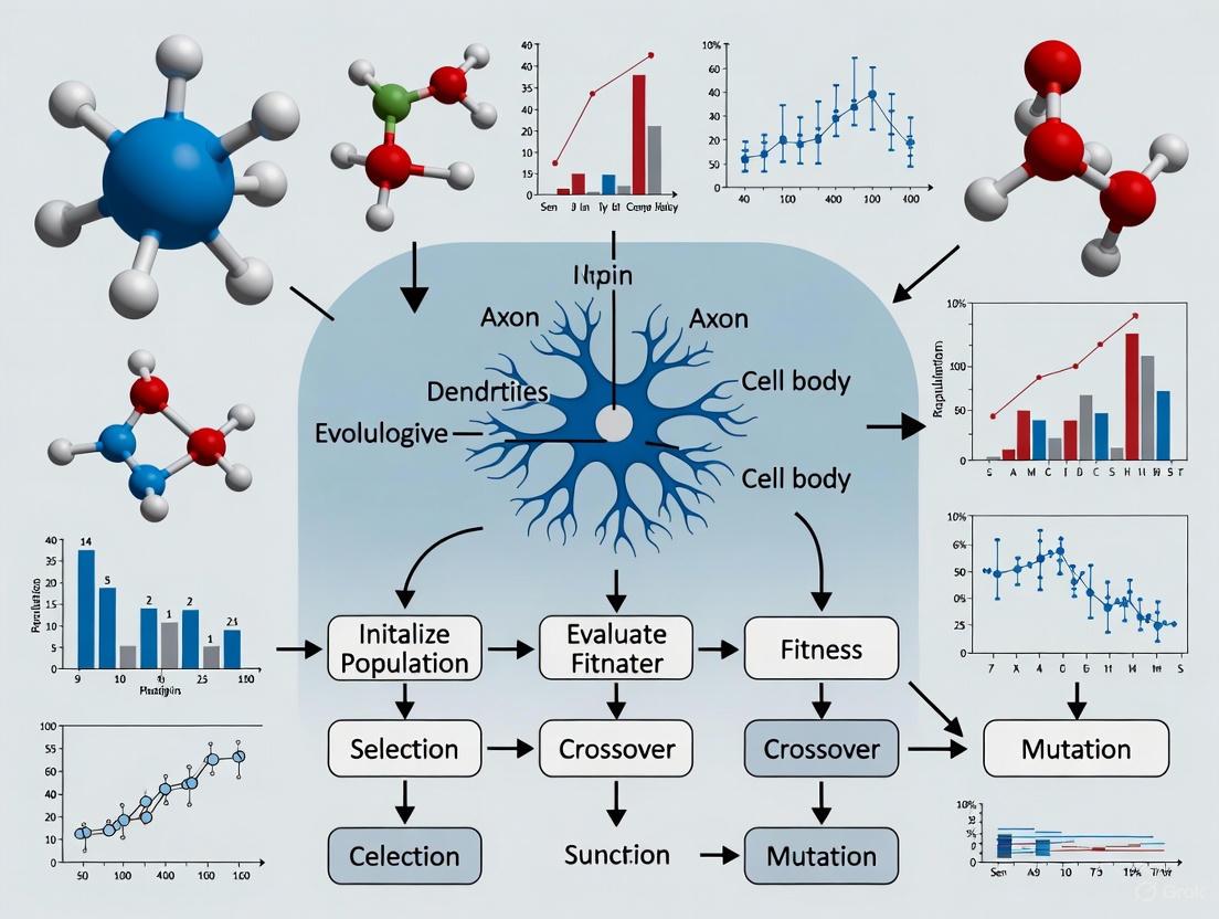
The following diagram illustrates the logical flow of a typical evolutionary algorithm applied to neuron model fitting.
Evolutionary Algorithms (EAs) represent a family of nature-inspired optimization techniques that have demonstrated remarkable effectiveness in tackling complex scientific computing problems, particularly in domains where traditional gradient-based methods struggle. These population-based metaheuristics are especially valuable for handling high-dimensional, non-convex, noisy, or multi-modal optimization landscapes commonly encountered in scientific research. Within neuroscience and drug development, EAs have become indispensable tools for parameter estimation in complex neuronal models, a process critical for understanding neural circuitry and neurological disease mechanisms.
The adaptation of EAs for scientific applications addresses several fundamental challenges in computational biology: poorly-characterized objective function landscapes, the presence of numerous local optima, and the need to integrate diverse experimental data types. By implementing biologically-inspired operations including mutation, crossover, and selection, EAs can efficiently explore vast parameter spaces while avoiding premature convergence to suboptimal solutions. For researchers fitting biophysical neuron models, these characteristics translate to an enhanced ability to determine the ion channel distributions and membrane properties that govern neuronal electrical behavior, ultimately supporting more accurate simulations of neural network dynamics.
This article focuses on three cornerstone EA variants—Genetic Algorithms (GAs), Differential Evolution (DE), and Evolution Strategies (ES)—that have demonstrated particular utility in scientific computing applications. We present a structured analysis of their operational principles, performance characteristics, and implementation protocols tailored to the specific requirements of neuronal model fitting, providing researchers with practical guidance for deploying these powerful optimization techniques in their computational workflows.
Algorithmic Foundations and Comparative Analysis
Genetic Algorithms (GAs)
Genetic Algorithms operate on a population of candidate solutions, typically encoded as fixed-length chromosomes, through selection, crossover, and mutation operations. The fundamental GA workflow begins with population initialization, followed by iterative fitness evaluation and application of genetic operators to create successive generations. Selection mechanisms favor individuals with higher fitness—those that better solve the optimization problem—while crossover recombines genetic material from parent solutions and mutation introduces random perturbations to maintain population diversity [6].
In neuronal model fitting, GAs excel at exploring discrete and continuous parameter spaces simultaneously, making them suitable for optimizing both model topology and kinetic parameters. Their representation flexibility allows researchers to encode various model aspects, including ion channel densities, synaptic weights, and morphological parameters within a unified chromosome representation. The main advantage of GAs lies in their global search capabilities, which help identify promising regions of complex parameter spaces before fine-tuning solutions [6].
Differential Evolution (DE)
Differential Evolution specializes in optimizing continuous parameters through vector-based operations, making it particularly well-suited for kinetic parameter estimation in neuronal models. DE generates new candidate solutions by combining scaled differences between population members with existing solutions, creating a search behavior that automatically adapts to the objective function landscape. The algorithm's performance heavily depends on its mutation strategy and control parameters (mutation factor and crossover rate), which determine the evolutionary scale of the search process [7].
Recent advances in DE include the Evolutionary Scale Adaptation DE (ESADE), which introduces a successful scale estimation mechanism that utilizes feedback from trial vectors to dynamically adjust the evolutionary scale. This adaptation allows ESADE to match search requirements across different evolutionary stages, employing either small or large evolutionary steps as appropriate [7]. For neuronal model fitting, this adaptability translates to more efficient exploration of high-dimensional parameter spaces, as demonstrated by ESADE's superior performance on benchmark functions and real-world optimization problems compared to classical DE approaches [7].
Evolution Strategies (ES)
Evolution Strategies distinguish themselves through their self-adaptive mechanism for strategy parameters, particularly the mutation strengths applied to different dimensions. Modern ES variants, particularly the Covariance Matrix Adaptation ES (CMA-ES), implement a sophisticated adaptation of the covariance matrix that determines the mutation distribution, effectively learning second-order information about the objective function topology [6] [8].
The CMA-ES algorithm has emerged as a state-of-the-art approach for complex optimization problems in scientific computing due to its invariance to problem scaling and rotation. Its ability to automatically adapt the search distribution to the local objective function landscape makes it exceptionally effective for ill-conditioned problems where parameters exhibit different sensitivities and strong correlations [6] [8]. In neuronal model fitting, this capability is invaluable for handling the disparate time scales and parameter interactions characteristic of ion channel kinetics and synaptic transmission mechanisms.
Table 1: Comparative Analysis of Key Evolutionary Algorithm Variants
| Algorithm | Representation | Key Operators | Adaptation Mechanism | Strengths in Neuronal Model Fitting |
|---|---|---|---|---|
| Genetic Algorithms (GAs) | Binary, Integer, Real-valued | Selection, Crossover, Mutation | Parameter control through algorithm tuning | Flexible representation for mixed parameters; Effective global search |
| Differential Evolution (DE) | Real-valued vector | Mutation, Crossover | Evolutionary scale adaptation [7] | Efficient continuous optimization; Self-adaptive step sizes |
| Evolution Strategies (ES) | Real-valued vector | Mutation, Selection | Covariance matrix adaptation [6] | Handles parameter correlations; Invariant to problem transformations |
Application Protocols for Neuronal Model Fitting
Problem Formulation and Fitness Function Design
The foundational step in applying EAs to neuronal model fitting involves formulating an appropriate fitness function that quantifies the discrepancy between model output and experimental data. For biophysical neuronal models, this typically involves comparing simulated membrane potentials with electrophysiological recordings across multiple stimulation protocols. The fitness function often incorporates multiple objective components, including features such as action potential timing, shape characteristics, firing rates, and subthreshold dynamics [9].
A practical approach implements fitness computation through electrophysiological feature extraction, where specific characteristics of neuronal activity are quantified and compared. The fitness (F) can be represented as a weighted sum of individual feature discrepancies: F = ∑wi⋅|fisimulated - fiexperimental|, where wi represents the weight assigned to feature i based on its importance and reliability. This multi-objective formulation ensures that the optimization process captures the essential electrophysiological properties of the target neuron rather than simply minimizing point-wise differences in membrane potential [9].
Implementation Framework for High-Performance Computing
Modern neuronal model fitting with EAs demands substantial computational resources, necessitating implementation strategies that leverage high-performance computing architectures. The NeuroGPU-EA framework demonstrates an optimized approach that utilizes both CPUs and GPUs concurrently to accelerate the simulate-evaluate loop central to evolutionary optimization [9]. This implementation employs three scaling strategies to manage computational resources efficiently:
- Compute Fixed and Problem Scales: The number of neuron models in the EA population increases while computing resources remain fixed
- Strong Scaling (Compute Scales and Problem Fixed): Computing resources increase while the problem size remains constant
- Weak Scaling (Compute Scales and Problem Scales): Both computing resources and problem size increase at a fixed ratio [9]
This framework achieves a 10× performance improvement over CPU-based EA implementations by parallelizing neuronal simulations across GPU resources and efficiently distributing fitness evaluations across available computing nodes. The implementation demonstrates logarithmic cost scaling when increasing the number of stimuli used in the fitting procedure, making it practical to incorporate diverse experimental protocols that enhance model robustness and generalizability [9].
Specialized EA Variants for Sparse and High-Dimensional Problems
Large-scale sparse multi-objective optimization problems (LSSMOPs) frequently arise in neuronal modeling contexts, particularly when optimizing network connectivity or channel distributions where most parameters should be zero. Standard EAs perform undifferentiated operations on all decision variables, reducing search efficiency and producing solutions that fail to meet sparsity requirements [10]. The SparseEA algorithm addresses this challenge through a bi-level encoding strategy that represents solutions using both continuous decision variables and binary mask vectors that control parameter sparsity [10].
The enhanced SparseEA-AGDS framework introduces an adaptive genetic operator and dynamic scoring mechanism that adjusts crossover and mutation probabilities based on non-dominated layer levels of individuals. This approach updates decision variable scores iteratively, enabling superior individuals to receive increased genetic opportunities while maintaining solution sparsity [10]. For neuronal model fitting, this translates to more efficient optimization of high-dimensional parameter spaces where only a subset of parameters significantly influences model behavior, such as when determining the minimal set of ion channel types needed to reproduce specific electrophysiological phenotypes.
Table 2: Performance Comparison of EA Variants on Scientific Computing Tasks
| Algorithm | Parameter Recovery Accuracy | Computational Efficiency | Noise Resilience | Implementation Complexity |
|---|---|---|---|---|
| CMA-ES | High for correlated parameters [8] | Moderate to High [8] | Moderate | High |
| Differential Evolution | Variable (problem-dependent) [8] | High [7] | Low to Moderate | Low |
| SparseEA-AGDS | High for sparse problems [10] | High for high-dimensional problems [10] | Not Reported | Moderate |
| Genetic Algorithms | Moderate | Low to Moderate | Moderate | Low |
Experimental Protocols and Benchmarking
Protocol 1: Kinetic Parameter Estimation for Neural Models
Objective: Determine the kinetic parameters of ion channel and synaptic models that minimize the discrepancy between simulated and experimental neuronal activity.
Materials and Reagents:
- Experimental electrophysiology data: Voltage clamp, current clamp, or dynamic clamp recordings from target neurons
- Biophysical neuron model: Compartmental model implemented in simulation environments (NEURON, GENESIS, Brian)
- Computational resources: Multi-core CPUs or GPU acceleration for parallel simulation
Procedure:
- Parameter Boundary Definition: Establish physiologically plausible lower and upper bounds for each kinetic parameter based on literature and experimental constraints
- EA Initialization:
- Population size: 100-1000 individuals (increases with parameter dimension)
- Mutation strategy: DE/rand/1/bin for DE or Gaussian mutation for ES
- Crossover: Binomial for DE, simulated binary for real-coded GA
- Parallel Evaluation:
- Distribute population individuals across available computing cores
- Run neuronal simulations with identical stimulus protocols
- Extract features from simulated voltage traces (action potential properties, firing rates, etc.)
- Fitness Computation: Calculate multi-objective fitness incorporating weighted feature differences
- Evolutionary Operations: Apply selection, mutation, and crossover to generate offspring population
- Termination Check: Continue until fitness improvement falls below threshold or maximum generations reached
Validation: Assess model generalizability using novel stimulus patterns not included in the fitting process [9] [8]
Protocol 2: Benchmarking EA Performance for Specific Reaction Kinetics
Objective: Evaluate the effectiveness of different EA variants for estimating parameters of specific biochemical reaction kinetics relevant to neuronal signaling.
Experimental Design:
- Kinetic Formulations: Test across multiple reaction kinetics types:
- Generalized Mass Action (GMA)
- Michaelis-Menten kinetics
- Linear-logarithmic (Linlog) kinetics
- Noise Conditions: Evaluate performance under varying levels of measurement noise (0-20% coefficient of variation)
- Performance Metrics:
- Parameter recovery accuracy (mean squared error between true and estimated parameters)
- Computational cost (function evaluations and processing time)
- Convergence reliability (success rate across multiple independent runs)
Implementation Notes:
- For GMA kinetics, CMAES requires fewer computational resources while maintaining accuracy [8]
- For Michaelis-Menten kinetics, G3PCX achieves superior performance with substantial computational savings [8]
- Under high noise conditions, SRES and ISRES demonstrate improved reliability for GMA kinetics at higher computational cost [8]
Table 3: Essential Research Reagents and Computational Tools for EA-Based Neuronal Model Fitting
| Tool/Resource | Function | Application Notes |
|---|---|---|
| NEURON Simulation Environment [9] | Simulates electrical activity of neurons | Industry standard for compartmental modeling; GPU acceleration available |
| CoreNeuron [9] | Optimized simulator for HPC systems | Used in NeuroGPU-EA for massively parallel simulation |
| Electrophysiological Feature Extraction Libraries [9] | Quantifies spike train characteristics | Critical for fitness computation; implementations vary in computational efficiency |
| CMA-ES Implementation [8] | Advanced evolution strategy | Preferred for correlated parameter spaces; self-adaptive |
| SparseEA-AGDS Framework [10] | Handles large-scale sparse optimization | Essential for connectivity optimization and channel distribution problems |
| High-Performance Computing Cluster [9] | Provides parallel processing resources | Enables weak and strong scaling experiments; reduces fitting time from weeks to hours |
Evolutionary Algorithms provide a powerful, flexible framework for addressing the complex optimization challenges inherent in neuronal model fitting. The three primary variants discussed—Genetic Algorithms, Differential Evolution, and Evolution Strategies—each offer distinct advantages for different aspects of the parameter estimation problem. GAs provide representation flexibility, DE offers efficient continuous optimization, and ES delivers sophisticated adaptation to problem geometry. The emergence of specialized variants like ESADE and SparseEA-AGDS further extends these capabilities to handle specific challenges such as evolutionary scale adaptation and high-dimensional sparse optimization.
Future developments in EA research will likely focus on enhanced hybridization with local search methods, improved adaptation mechanisms, and tighter integration with machine learning approaches. For neuronal model fitting specifically, we anticipate increased emphasis on multi-objective optimization that simultaneously fits multiple electrophysiological phenotypes and experimental conditions. As computational resources continue to grow, EAs will play an increasingly central role in building biologically-realistic neuronal models that bridge molecular mechanisms and system-level neural computations, ultimately advancing our understanding of brain function and dysfunction.
Fitting computational models to neuronal data is a cornerstone of modern neuroscience, essential for understanding brain function and dysfunction. This process, however, is fraught with challenges due to the inherently nonlinear nature of neuronal dynamics and the high-dimensional parameter spaces of biologically realistic models. Traditional optimization methods, particularly gradient-based approaches, often struggle with these complexities, converging to suboptimal solutions or requiring extensive manual intervention. Evolutionary algorithms (EAs) have emerged as a powerful alternative, demonstrating superior performance in navigating complex error landscapes and finding near-optimal parameter sets where other methods fail. This application note details the theoretical foundations, practical protocols, and specific advantages of using EAs for neuron model fitting within a research context, providing scientists with the tools to implement these methods effectively.
Comparative Analysis of Fitting Algorithms
The choice of optimization algorithm critically impacts the success and efficiency of neuron model fitting. The table below summarizes the key characteristics of different algorithm classes.
Table 1: Comparison of Optimization Algorithms for Neuron Model Fitting
| Algorithm Class | Key Mechanism | Handling of Local Minima | Scalability to High Dimensions | Best-Suited Application Context |
|---|---|---|---|---|
| Gradient Following (GF) | Follows error gradient downhill [11] | Poor; highly susceptible [11] | Moderate; can be computationally expensive [11] | Models with smooth, convex error surfaces and good initial parameter estimates [11] |
| Evolutionary Algorithms (EA) | Population-based stochastic search [11] [2] | Excellent; avoids entrapment via global search [11] | High; effective for 100+ parameters [12] | Complex, nonlinear models with noisy data and unknown initial parameters [11] [12] |
| Markov Chain Monte Carlo (MCMC) | Bayesian sampling of posterior distribution [13] | Good; explores multiple modes [13] | Moderate; can be computationally intensive [13] | Problems requiring uncertainty quantification and full posterior analysis [13] |
| Bayesian Optimization (BO) | Builds probabilistic model of objective function [12] | Good for low-dimensional spaces | Lower; performance degrades with increasing dimensions [12] | Expensive black-box functions with small parameter sets (e.g., <20) [12] |
Quantitative evidence underscores the strengths of EAs. A study fitting a 9-parameter model of a visual neuron found that while a GF method converged rapidly, it was "highly susceptible to the effects of local minima" and produced poor fits unless initial parameters were "already very good." Conversely, the EA "found better solutions in nearly all cases" and its performance was "independent of the starting parameters" [11]. In high-dimensional settings, such as optimizing a whole-brain model with ~100 region-specific parameters, the Covariance Matrix Adaptation Evolution Strategy (CMA-ES), a sophisticated EA, significantly improved the goodness-of-fit (GoF) compared to low-dimensional scenarios [12].
Essential Research Reagents and Computational Tools
Successful implementation of EA-based fitting requires a suite of computational tools and models. The following table catalogues key "research reagents" for this domain.
Table 2: Key Research Reagent Solutions for EA-based Neuron Model Fitting
| Reagent / Tool Name | Type | Primary Function in Workflow | Example Use-Case / Notes |
|---|---|---|---|
| Hodgkin-Huxley (HH) Model [13] [14] | Biophysically Detailed Neuron Model | Serves as a high-fidelity forward model for simulating action potentials; parameters (e.g., conductance densities) are fit to data. | An 8-channel HH model was used to demonstrate parameter inference via MCMC, highlighting non-uniqueness [13]. |
| McIntyre-Richardson-Grill (MRG) Model [15] | Biophysically Detailed Axon Model | Gold-standard model for predicting myelinated peripheral nerve fiber responses to electrical stimulation. | Used as a benchmark for validating the surrogate S-MF model; provides ground-truth data for fitting [15]. |
| Surrogate Myelinated Fiber (S-MF) [15] | Simplified, GPU-Accelerated Surrogate Model | Massively parallel, efficient emulator of the MRG model; enables rapid EA-based parameter searches and optimization. | Achieved >2,000x speedup over NEURON model, enabling large-scale parameter sweeps for VNS [15]. |
| NEURON Simulation Environment [15] | Industry-Standard Neural Simulator | Platform for running biophysically realistic simulations; used to generate training data for surrogates or as a forward model. | CPU-based; the only platform supporting extracellular voltages in complex fiber models [15]. |
| AxonML Framework [15] | Computational Framework | Implements, parameterizes, and efficiently executes GPU-based models like S-MF for high-throughput simulation and optimization. | Facilitates gradient-free and gradient-based optimization of stimulation parameters [15]. |
Detailed Experimental Protocols
Protocol 1: Fitting a Filter-Based Visual Neuron Model using EA
This protocol is adapted from a study that successfully employed an EA to fit a 9-parameter model to data from 107 macaque V1 neurons [11].
Workflow Overview
Step-by-Step Procedure
Problem Formulation:
- Define the Forward Model: Implement the mathematical model of the visual neuron. In the referenced study, this was a 9-parameter, nonlinear, filter-based model.
- Choose a Fitness Metric: Select a metric to quantify the discrepancy between model output and empirical data. Common choices include:
- Sum of Squared Residuals (SSQ): A standard distance-based measure [11].
- Variance Explained (R²): The percentage of variance in the data accounted for by the model. The error term is 1 - R² [11].
- Ratio within Confidence Interval (RCI): The percentage of model outputs falling within the confidence intervals of the data points. The error term is 1 - RCI [11].
EA Configuration:
- Initialize Population: Generate a population of candidate solutions (individuals), each being a random vector of the 9 model parameters within physiologically plausible bounds.
- Set EA Hyperparameters: Define population size (e.g., 100-500), number of generations, mutation rate, crossover rate, and selection strategy (e.g., tournament selection).
Iterative Optimization:
- Evaluate Fitness: For each individual in the population, run the forward model with its parameters and calculate the fitness (error) against the target neuronal data.
- Select Parents: Probabilistically select individuals from the current population to become parents, favoring those with higher fitness (lower error).
- Create Offspring: Apply genetic operators (crossover and mutation) to the parents to generate a new population of offspring.
- Repeat: Continue the evaluate-select-create cycle for hundreds or thousands of generations until a stopping criterion is met (e.g., fitness plateaus, maximum generations reached).
Validation and Analysis:
- Solution Quality: The EA is expected to converge on a parameter set that provides a fit close to the global optimum, independent of the initial parameter guesses [11].
- Comparison: Validate the EA's performance by comparing its final fitness and the biological plausibility of the found parameters against solutions obtained from GF methods from multiple random starting points.
Protocol 2: High-Dimensional Parameter Optimization for Whole-Brain Modeling
This protocol outlines the use of CMA-ES for fitting a whole-brain model of coupled oscillators with region-specific parameters, optimizing up to 103 parameters simultaneously for 272 subjects [12].
Workflow Overview
Step-by-Step Procedure
Model and Objective Definition:
- Whole-Brain Model: Implement a dynamical whole-brain model, such as a network of coupled phase oscillators, where each brain region has one or more local parameters (e.g., coupling strength, oscillation frequency).
- Objective Function: The goal is to maximize the correlation between the simulated functional connectivity (sFC) matrix and the empirical FC (eFC) matrix derived from subject resting-state fMRI data. Fitness is typically defined as the Pearson correlation coefficient between the upper triangles of the sFC and eFC matrices.
CMA-ES Setup:
- Initialize Algorithm: Initialize the CMA-ES with a mean vector (initial guess for the parameter set) and a covariance matrix. The covariance matrix is initially set to explore a wide area of the high-dimensional parameter space.
- Parameter Bounds: Define lower and upper bounds for all parameters based on biological constraints.
High-Throughput Optimization:
- Sample Population: In each generation, sample a population of candidate parameter vectors from a multivariate normal distribution defined by the current mean and covariance.
- Parallel Evaluation: For each candidate parameter vector, run the whole-brain simulation to generate time series data, calculate the sFC, and then compute its fitness (correlation with eFC). Leverage high-performance computing resources to evaluate populations in parallel.
- Algorithm Update: The CMA-ES algorithm ranks the candidate solutions, and then updates its internal state (the mean and covariance matrix) to bias the search towards regions of higher fitness in the subsequent generation.
Post-Optimization Analysis:
- Goodness-of-Fit (GoF): The primary output is the maximized correlation between sFC and eFC. Studies report that optimization in high-dimensional spaces "improved considerably" the GoF [12].
- Parameter Reliability: Analyze the variability of the optimized parameters across multiple independent runs for the same subject. Note that parameters may show "increased variability within subjects and reduced reliability across repeated optimization runs," but the resulting sFC and GoF remain stable and reliable [12].
- Application: Use the optimized parameters or the GoF as features for downstream analyses, such as classifying subject sex or predicting behavioral measures [12].
Evolutionary algorithms represent a robust, powerful, and often necessary approach for fitting the complex, high-dimensional models that are central to modern computational neuroscience. Their ability to avoid local minima, handle nonlinearity without gradient information, and scale to problems with hundreds of parameters makes them uniquely suited for personalizing whole-brain models and inferring parameters for biophysically detailed neuron models. While the computational cost per function evaluation can be high, the advent of surrogate models and high-performance computing platforms is mitigating this limitation. By adopting the protocols and insights outlined in this application note, researchers can effectively leverage EAs to uncover the underlying principles of neural dynamics.
Quantitative Systems Pharmacology (QSP) has emerged as a powerful mechanistic modeling approach that integrates diverse biological, physiological, and pharmacological data to predict drug interactions and clinical outcomes [16] [17]. As the field matures, its applications have expanded beyond research and development into decision-making and regulatory arenas, with the FDA reporting approximately 60 QSP submissions in 2020 alone [18]. QSP establishes a conceptual, integrative framework rather than a specific computational methodology, combining elements of systems biology, systems pharmacology, systems physiology, and data science under the umbrella of dynamic systems theory [16].
The integration of Artificial Intelligence (AI) and large language models (LLMs) is now transforming QSP by enhancing model generation, interpretability, and reproducibility [19] [20]. Evolutionary Algorithms (EAs) represent a particularly promising branch of computational intelligence that can address complex optimization challenges in QSP model development, especially in parameter estimation and model calibration. This framework outlines specific protocols for aligning EA objectives with Model-Informed Drug Development (MIDD) goals to enhance QSP model qualification and regulatory acceptance.
Background
The QSP Workflow and Its Challenges
QSP model development follows a progressive maturation workflow encompassing several stages [21]. This begins with project definition and needs assessment, proceeds through biological knowledge review and model structuring, continues with mathematical formulation and parameterization, and concludes with model qualification and application [21] [19]. Throughout this process, modelers face persistent operational challenges including labor-intensive literature curation, parameter uncertainty, lack of standardized validation protocols, and long turnaround times [19].
Table 1: Key Challenges in QSP Workflow Execution
| Stage | Primary Activities | Associated Challenges |
|---|---|---|
| Project Definition | Articulation of scientific hypotheses and therapeutic endpoints | Limited biological understanding; absence of formal requirements documentation |
| Biological Knowledge Review | Systematic literature curation and pathway identification | Heterogeneous data quality; labor-intensive manual curation processes |
| Model Structure Development | Translation of biological networks to mathematical framework | Structural inconsistencies; limited reusability of existing components |
| Mathematical Formulation | Parameter identification and estimation | Parameter uncertainty; sparse experimental data for calibration |
| Model Qualification | Validation against clinical data; sensitivity analysis | Lack of standardized validation protocols; risk of overfitting |
Evolutionary Algorithms in QSP Context
Evolutionary Algorithms represent a family of population-based optimization techniques inspired by biological evolution, including selection, crossover, and mutation operations. In QSP, EAs are particularly valuable for addressing high-dimensional, non-convex optimization problems where traditional gradient-based methods struggle. Their population-based nature enables global exploration of parameter spaces while handling complex constraints commonly encountered in biological systems.
Framework for EA-QSP Integration
Conceptual Alignment
The successful integration of EAs within QSP requires careful alignment between algorithmic objectives and MIDD goals. This alignment ensures that computational efficiency translates to meaningful pharmacological insights and decision support. EA objectives must be formulated to directly address the core challenges of QSP model development, particularly parameter identifiability, validation against heterogeneous data sources, and clinical translation.
Technical Implementation Framework
The technical integration of EAs within QSP workflows requires a structured approach to algorithm selection, objective function formulation, and constraint handling. This framework leverages EAs as global optimizers for parameter estimation and model calibration across multiple data modalities and experimental conditions.
Table 2: EA Configuration for QSP Parameter Estimation
| EA Component | QSP Implementation | MIDD Alignment |
|---|---|---|
| Fitness Function | Multi-objective function balancing agreement with training data and physiological plausibility | Ensures models are both accurate and biologically interpretable for regulatory review |
| Representation | Real-valued parameter vectors with logarithmic scaling for kinetic parameters | Accommodates parameters spanning multiple orders of magnitude common in biological systems |
| Selection | Tournament selection with elitism preservation | Maintains diversity while preserving best-performing parameter sets |
| Genetic Operators | Simulated binary crossover with polynomial mutation | Enables efficient exploration of high-dimensional parameter spaces |
| Constraint Handling | Penalty functions for physiologically implausible parameter regions | Ensures parameter estimates remain within biologically meaningful ranges |
Experimental Protocols
Protocol 1: EA-Driven QSP Model Calibration
Purpose: To establish a robust methodology for calibrating QSP models using evolutionary algorithms that ensures parameter identifiability and physiological plausibility.
Materials and Reagents:
- Biological system data (e.g., pharmacokinetic, pharmacodynamic, biomarker data)
- Computational resources (multi-core processors, high-performance computing cluster)
- Software platforms (MATLAB, R, Python with DEAP or similar EA libraries)
- QSP model structure (ordinary differential equations, algebraic equations)
Procedure:
- Problem Formulation:
- Define the parameter estimation problem with identified decision variables
- Establish parameter bounds based on physiological constraints and prior knowledge
- Formulate multi-objective fitness function incorporating weighted data agreement metrics
EA Configuration:
- Initialize population of candidate parameter vectors using Latin Hypercube Sampling
- Set algorithm parameters: population size (100-500), generations (1000-5000), crossover (0.8-0.95) and mutation rates (1/n, where n=number of parameters)
- Implement niching or crowding mechanisms to maintain population diversity
Optimization Execution:
- Execute EA optimization with parallel fitness evaluation
- Implement termination criteria based on convergence metrics or maximum generations
- Store complete optimization trajectory for post-hoc analysis
Validation and Analysis:
- Perform profile likelihood analysis on optimized parameter sets
- Conduct global sensitivity analysis using Sobol or Morris methods
- Validate model predictions against held-out experimental data
Expected Outcomes: A calibrated QSP model with quantified parameter uncertainty, suitable for predictive simulations and regulatory submission support.
Protocol 2: EA-Enhanced Virtual Population Generation
Purpose: To generate clinically plausible virtual patient populations that capture inter-individual variability using evolutionary algorithms.
Materials and Reagents:
- Population-level clinical data
- Covariate distribution information
- QSP model with identified sources of variability
- Statistical software for distribution fitting
Procedure:
- Variability Source Identification:
- Determine which model parameters contribute to inter-individual variability
- Establish correlation structure between parameters based on physiological knowledge
- Define target distributions for clinically observable biomarkers
EA Optimization Setup:
- Formulate fitness function measuring distance between virtual population statistics and clinical data summaries
- Define decision variables as parameters of multivariate distributions for model parameters
- Set constraints to maintain physiological plausibility of generated individuals
Population Evolution:
- Initialize candidate distribution parameters
- Iteratively refine distribution parameters using EA optimization
- Apply niching techniques to capture multiple subpopulations if present
Virtual Population Validation:
- Assess reproduction of target clinical statistics
- Verify preservation of parameter correlations
- Confirm coverage of clinically observed subpopulations
Expected Outcomes: A virtual population that accurately reflects clinical variability for use in clinical trial simulations and dose regimen optimization.
The Scientist's Toolkit
Table 3: Research Reagent Solutions for EA-QSP Integration
| Tool Category | Specific Tools | Function in EA-QSP Workflow |
|---|---|---|
| Optimization Frameworks | DEAP (Python), MATLAB Global Optimization Toolbox, R GA Package | Provide evolutionary algorithm implementations for parameter estimation and optimization |
| Modeling & Simulation | MATLAB/SimBiology, R/xQSP, Julia/SciML | Enable QSP model development, simulation, and parameter sensitivity analysis |
| Data Curation & Integration | AI-augmented platforms (QSP-Copilot) [19], Natural language processing tools | Accelerate literature curation and data extraction from heterogeneous sources |
| High-Performance Computing | AWS, Azure, Google Cloud, SLURM clusters | Enable parallel fitness evaluation and computationally intensive EA runs |
| Visualization & Analysis | MATLAB Plotting, R/ggplot2, Python/Matplotlib | Facilitate visualization of optimization trajectories and model performance |
| Model Qualification | Profile Likelihood Implementation, Sobol Sensitivity Analysis | Support model validation and identifiability analysis for regulatory submissions |
Application Case Study: CRISPR-Cas Therapy Translation
To demonstrate the practical implementation of this framework, we applied EA-driven QSP modeling to the translation of in-vivo CRISPR-Cas therapy [22]. This novel therapeutic modality involves complex pharmacokinetic/pharmacodynamic relationships spanning multiple biological scales.
Implementation: We developed a QSP model incorporating mechanisms post-IV injection including LNP binding to opsonins, phagocytosis, cellular internalization, mRNA translation, and gene editing. Evolutionary algorithms were employed to estimate key parameters including the rate of internalization in the interstitial layer (0.039 1/h in NHP vs. 0.007 1/h in humans) and the rate of exocytosis (6.84 1/h in mouse, 2690 1/h in NHP, and 775 1/h in humans) [22].
Results: The EA-optimized model successfully characterized biodistribution and dose-exposure relationships across species, demonstrating the framework's utility in facilitating the discovery and development of novel therapeutic agents. Monte Carlo simulations using the calibrated model accurately predicted serum TTR reduction in patients, supporting first-in-human dose selection.
The integration of evolutionary algorithms within Quantitative Systems Pharmacology represents a powerful approach to addressing key challenges in model development and qualification. By formally aligning EA objectives with MIDD goals, this framework enhances the efficiency, robustness, and regulatory acceptance of QSP models. The provided protocols and toolkit offer practical guidance for implementation across various therapeutic areas, potentially reducing model development time by approximately 40% through automation of routine tasks [19]. As QSP continues to evolve as a critical component of model-informed drug development, evolutionary algorithms will play an increasingly important role in harnessing the full potential of these complex mechanistic models to advance therapeutic development.
Building Your EA Pipeline: A Step-by-Step Protocol for Neuron Model Optimization
In computational neuroscience, the fitness function serves as the crucial bridge between a neurobiological hypothesis and a functional, optimized model. It is the mathematical embodiment of the research question, guiding evolutionary algorithms (EAs) to evolve in-silico neurons that replicate empirical observations. A well-formulated fitness function ensures that the evolutionary search explores parameter spaces that are not only computationally optimal but also neurobiologically plausible. This protocol outlines the principles and procedures for constructing such fitness functions, enabling researchers to effectively translate complex neurobiological concepts into quantifiable optimization targets for neuron model fitting.
Core Components of a Fitness Function for Neuron Model Fitting
A fitness function for biophysical neuron model fitting typically integrates multiple components to ensure the model accurately reproduces empirical electrophysiological data. The structure balances several competing objectives to achieve biological realism.
Table 1: Core Components of a Fitness Function for Neuron Model Fitting
| Component Category | Specific Metric | Neurobiological Interpretation | Mathematical Formulation Examples |
|---|---|---|---|
| Distance-Based Measures | Sum of Squared Residuals (SSQ) / Root-Mean-Squared (RMS) Error | Quantifies overall deviation of model output from experimental voltage traces. [11] | SSQ = Σ(Experimental_V - Model_V)² |
| Mean Squared Error (MSE) | Average squared difference, independent of data point number. [11] | MSE = SSQ / N (N = number of data points) |
|
| Correlation-Based Measures | Variance Explained (R²) | Percentage of variance in experimental data accounted for by the model; sensitive to response shape. [11] | R² = 1 - [SSQ / Σ(Experimental_V - Mean_V)²] |
| Criteria-Based Measures | Ratio within Confidence Intervals (RCI) | Proportion of model outputs falling within experimental confidence intervals; intuitively interpretable. [11] | RCI = (Count[Model_V within CI] / N); Error = 1 - RCI |
| Biophysical Constraints | Channel Kinetics & Properties | Ensures inferred ion channel parameters (e.g., conductance, kinetics) align with prior biological knowledge. [1] | Penalty terms for parameters outside physiologically plausible ranges. |
Experimental Protocols for Fitness Function Formulation
Protocol: Multi-Objective Formulation and Calibration
Objective: To construct a composite fitness function that robustly balances multiple, potentially competing, error measures for effective evolutionary search.
- Identify Primary Data Features: Determine the key electrophysiological features essential for testing your hypothesis (e.g., resting membrane potential, spike rate, spike width, adaptation index, sag amplitude, rebound depolarization).
- Select Error Metrics: Choose a primary error metric (e.g., SSQ for overall fit) and one or two secondary metrics (e.g., R² for shape, RCI for confidence) from Table 1. [11]
- Define Sub-Objectives: Formulate the optimization as a multi-objective problem, aiming to minimize all selected error metrics simultaneously.
- Weight Assignment (if scalarizing): If using a weighted sum approach, assign initial weights heuristically based on feature importance. For example:
- Weight for spike timing error: 0.6
- Weight for spike height error: 0.3
- Weight for resting potential error: 0.1
- Iterative Calibration: Execute the EA with the initial weights. Analyze the resulting models. If a specific feature is not fitting well, incrementally increase its weight and re-run. Utilize algorithms like the Indicator-Based Evolutionary Algorithm (IBEA) capable of handling multiple objectives without manual weight tuning. [9]
Protocol: Handling Noisy Electrophysiological Data
Objective: To design a fitness function that is robust to inherent biological variability and measurement noise, preventing overfitting.
- Replicate Experimental Context: Incorporate multiple stimulus protocols (e.g., step currents, ramps, noise injections) into the fitness evaluation, as variability across stimuli can help the EA discern correct underlying parameters. [9]
- Utilize Feature-Based Fitness: Instead of relying solely on point-by-point voltage comparisons (e.g., SSQ), extract and compare specific features from the voltage trace. This approach is less sensitive to high-frequency noise.
- Algorithm Selection for Noise: For problems with significant measurement noise, consider evolutionary strategies (ES) known for noise resilience, such as SRES (Stochastic Ranking Evolutionary Strategy) or ISRES (Improved SRES), as they can perform more reliably than other algorithms like CMA-ES in these conditions. [8]
- Regularization: Add penalty terms to the fitness function that discourage overly complex solutions or parameters that deviate far from known biological ranges, thus constraining the search to physiologically plausible models. [11] [1]
Optimization Methods and Algorithm Selection
Selecting an appropriate evolutionary algorithm is critical, as performance varies significantly with problem structure, dimensionality, and the presence of noise.
Table 2: Evolutionary Algorithm Performance for Neuron Model Fitting
| Algorithm | Best Suited For | Performance & Characteristics | Considerations |
|---|---|---|---|
| CMA-ES (Covariance Matrix Adaptation Evolution Strategy) | Low-noise problems; GMA and Linlog kinetics. [8] | High speed; requires a fraction of the computational cost of others in low-noise conditions. [8] | Performance can degrade with increasing measurement noise. [8] |
| SRES/ISRES (Stochastic Ranking ES) | Noisy data; GMA kinetics. [8] | Reliable performance under marked measurement noise. [8] | Higher computational cost compared to CMA-ES. [8] |
| G3PCX (Generalized Generation Gap) | Michaelis-Menten kinetics. [8] | Highly efficacious for parameter estimation; achieves numerous folds saving in computational cost. [8] | Performance may be formulation-specific. [8] |
| NeuroGPU-EA | High-dimensional parameter spaces; scalable fitting. | Leverages GPU parallelism; 10x faster than CPU-based EA on scaling benchmarks. [9] | Requires access to HPC resources with GPUs. [9] |
| Differential Evolution (DE) | General parameter estimation, but with limitations. | Used for estimating HH-model parameters from whole-cell recordings. [1] | Can show poor performance in some comparative studies, leading to its exclusion. [8] [1] |
The Scientist's Toolkit: Research Reagent Solutions
Table 3: Essential Software and Computational Tools
| Tool Name | Type/Category | Function in the Workflow |
|---|---|---|
| NEURON | Simulation Environment | Industry-standard software for simulating the electrical activity of neurons with complex morphologies and biophysics. [9] |
| CoreNeuron | GPU-Accelerated Simulator | Optimized version of NEURON for high-performance computing, enabling faster simulation on GPU nodes. [9] |
| ElectroPhysiomeGAN (EP-GAN) | Deep Generative Model | Instantly generates HH-model parameters from electrophysiological recordings, bypassing iterative optimization after training. [1] |
| IBEA (Indicator-Based Evolutionary Algorithm) | Optimization Algorithm | A multi-objective evolutionary algorithm used to find optimal trade-offs between multiple electrophysiological score functions. [9] |
| NeuroGPU-EA | Optimization Framework | A highly parallel evolutionary algorithm implementation designed for efficient model fitting on GPU-based supercomputers. [9] |
Workflow Visualization and Logical Pathways
The following diagram illustrates the end-to-end workflow for formulating a fitness function and applying an evolutionary algorithm to fit a neuron model.
Workflow for Evolutionary Neuron Model Fitting.
Translating a neurobiological hypothesis into an effective fitness function is a foundational step in evolutionary neuron model fitting. This process requires careful selection and combination of error metrics, informed calibration against experimental data, and the choice of an evolutionary algorithm suited to the problem's specific challenges. By adhering to the protocols and utilizing the tools outlined in this document, researchers can construct robust optimization frameworks that yield biophysically accurate and computationally efficient models, thereby providing deeper insights into neural function.
The accurate fitting of biophysical neuron models to experimental data is a cornerstone of computational neuroscience, enabling researchers to investigate the relationship between ion channel dynamics and neural function. Central to this optimization process is the evolutionary algorithm (EA), a prevalent method for navigating the high-dimensional parameter space of conductance-based models [23]. The performance and biological fidelity of these algorithms are critically dependent on the design of the fitness function, which quantifies the discrepancy between model output and empirical data. A well-constructed fitness function must achieve two primary objectives: it must faithfully incorporate a spectrum of electrophysiological features extracted from experimental recordings, and it must constrain the solution space to biologically plausible parameter sets. This application note details protocols for designing such fitness functions, structured to support the development of EAs for neuron model fitting. We provide a quantitative framework for feature selection, methodologies for multi-objective optimization, and strategies to embed biological constraints, thereby guiding researchers toward the creation of robust, generalizable, and physiologically relevant neuron models.
Core Principles of Fitness Function Design
The Multi-Objective Optimization Problem
Defining the fitness function for neuron model fitting is fundamentally a multi-objective optimization (MOO) problem [23]. The goal is to find parameter sets that present optimal trade-offs between multiple, often competing, electrophysiological objectives. A single neuron model can be evaluated against numerous features of its voltage trace, such as spike rate, latency, and adaptation. The EA searches for solutions that minimize a composite error across all these target features. This is frequently formulated using frameworks like the Indicator-Based Evolutionary Algorithm (IBEA), which allows for the simultaneous optimization of multiple criteria without collapsing them into a single, potentially misleading, scalar value [23] [24].
A significant challenge in this domain is the issue of degeneracy, where neurons with substantially different combinations of parameters can produce qualitatively similar electrophysiological responses [23] [1]. This implies that the mapping from parameter space to output space is not one-to-one. Consequently, a fitness function that focuses on a narrow set of features may find a solution that matches the target data but is biologically implausible. Therefore, the fitness function must be designed to navigate this degenerate landscape by incorporating a sufficiently diverse set of features and, where possible, including constraints that penalize parameter combinations falling outside physiologically realistic bounds.
From Localist to Distributed Representations
The evolution of neural network models in cognitive science offers a valuable analogy for fitness function design. Early localist models assigned a single cognitive element (e.g., a specific memory) to a single artificial neuron, a approach that is biologically unrealistic and does not account for distributed processing [25]. Similarly, a fitness function that relies on a single metric, such as overall spike count error, is often inadequate.
Modern approaches favor distributed representations, akin to those in auto-associative or attractor networks, where information is encoded across a population of neurons [25]. Translated to fitness function design, this means that the model's quality should be evaluated based on a distributed set of features that collectively define the neuron's electrophysiological identity. This approach ensures that the model captures the essence of the neural dynamics rather than merely matching one isolated aspect of its behavior. A multimodal optimizer, which explores a diverse population of model configurations for a single complex objective function, is an excellent tool for this purpose, as it directly embraces the distributed nature of the solution space [24].
Quantitative Electrophysiological Features for Fitness Evaluation
The accuracy of a fitted model is determined by how well it reproduces key electrophysiological features. The table below catalyses essential features that should be quantified from both experimental data and model simulations to compute the fitness score.
Table 1: Key Electrophysiological Features for Fitness Function Design
| Feature Category | Specific Feature | Biological Significance | Typical Scoring Function |
|---|---|---|---|
| Spike Train Characteristics | Firing Rate / I-F Curve | Neuronal excitability and input-output relationship [24] | Mean Squared Error (MSE) or Normalized Absolute Difference |
| Spike Latency (to first spike) | Timing precision and initial channel activation [24] | Absolute difference | |
| Interspike Intervals (ISI) | Spike frequency adaptation and bursting behavior [26] | Coefficient of variation or ISI histogram distance | |
| Action Potential Properties | Action Potential Amplitude | Na+ and K+ channel dynamics [26] | Absolute difference or MSE |
| Action Potential Half-Width | Spike duration and K+ channel kinetics [26] | Absolute difference or MSE | |
| After-Hyperpolarization (AHP) Depth | K+ channel-mediated hyperpolarization [26] | Absolute difference | |
| Subthreshold Dynamics | Resting Membrane Potential | Baseline ionic balance [27] | Absolute difference |
| Input Resistance | Passive membrane properties [27] | Absolute difference or normalized error | |
| Membrane Time Constant | Passive temporal integration [27] | Absolute difference | |
| Complex Patterns | Spike Frequency Adaptation | Ca2+-dependent K+ channel activity [24] | Exponential fit parameter comparison |
| Theta-Frequency Resonance (5-12 Hz) | Subthreshold resonance, important for information transmission [24] | Impedance amplitude profile (ZAP) response error |
The combination of these features into a single fitness function can be achieved through a weighted sum or a formal multi-objective optimization approach. The choice of features and their relative weights should be guided by the specific neuron type and the research questions being addressed.
Protocols for Fitness Function Implementation and Validation
Protocol: Constructing a Multi-Feature Fitness Function
This protocol outlines the steps for creating a comprehensive fitness function for optimizing a cerebellar granule cell (GrC) model, based on established methodologies [24].
Data Preparation and Feature Extraction:
- Stimulus Protocols: Apply a series of current injections to the biological neuron and the model. These should include:
- Feature Quantification: From the recorded and simulated voltage traces, extract the features listed in Table 1. For example, from step current responses, calculate the spike rate for each intensity to form the I-F curve, and measure the latency to the first spike.
Fitness Score Calculation:
- For each extracted feature ( i ), compute a normalized error ( Ei ) between the model output (( Mi )) and experimental target (( Ti )). A common method is the normalized absolute difference: ( Ei = |Mi - Ti| / |T_i| ).
- Aggregate Error: Combine the individual errors into a single fitness score (( F )) using a weighted sum: ( F = \sum{i=1}^{n} wi \cdot Ei ) where ( wi ) is the weight assigned to feature ( i ), reflecting its relative importance. The optimization aims to minimize ( F ).
- Alternative - Multi-Objective Formulation: Instead of a weighted sum, use a multi-objective EA (e.g., IBEA or NSGA-II) to treat each ( E_i ) as a separate objective. This yields a Pareto front of solutions representing optimal trade-offs between all features [23] [24].
Incorporating Biological Constraints:
- Parameter Bounds: Enforce hard constraints during the EA's mutation and crossover steps to keep all parameters (e.g., ion channel conductances) within physiologically realistic ranges [1].
- Soft Constraints via Penalty: Add a penalty term to the fitness score ( F ) if the model exhibits biologically impossible behavior, even if the feature match is good (e.g., negative membrane time constants or continuous spiking at rest).
Protocol: Validation and Generalization Testing
A fitted model must be validated to ensure it is not overfitted to the specific stimuli used for optimization and that it generalizes well [26].
- Benchmarking Performance: Compare the performance of your EA implementation against established benchmarks. This includes assessing strong scaling (fixed problem size with increasing computing resources) and weak scaling (problem size grows proportionally with resources) to evaluate computational efficiency [23].
- Validation with Unseen Stimuli: Test the optimized model against a completely different set of stimulation protocols (e.g., noisy current injections or ramp currents) that were not used during the fitting process. This assesses the model's ability to generalize beyond its training data.
- Population Generalization: To build a population of models (PoMs) that captures biological variability, use the same fitness function to optimize models against multiple experimental traces from different neurons. Assess the generalizability of the resulting population by testing how well it captures the statistical distribution of features in the biological population [27] [26]. A recent study demonstrated a 5-fold improvement in model generalizability using an automated workflow that includes rigorous validation [26].
The Scientist's Toolkit: Research Reagents and Solutions
Table 2: Essential Tools for EA-based Neuron Model Fitting
| Tool / Resource | Function | Application Note |
|---|---|---|
| BluePyOpt [23] [26] | A Python library for parameter optimization that implements various EAs (e.g., IBEA). | Provides the core optimization engine for defining parameters, fitness functions, and running the EA. |
| NEURON Simulator [23] [28] | A widely used environment for simulating biophysical neuron models. | Integrated with BluePyOpt to simulate the electrical activity of candidate models during fitness evaluation. |
| Arbor Simulator [26] | A high-performance, GPU-ready simulator for large-scale neural networks. | An alternative to NEURON, useful for accelerating simulations in computationally expensive optimizations. |
| BluePyEfel [26] | A Python library for extracting electrophysiological features from voltage traces. | Automates the calculation of features from both experimental and simulated data for fitness scoring. |
| Allen Brain Cell Types Database | A public repository containing electrophysiological recordings and neuronal morphologies. | A source of experimental data for defining target features for optimization, especially for cortical neurons. |
| DEAP Framework [23] | A general-purpose Evolutionary Computation framework in Python. | Can be used to build custom EAs if a pre-packaged solution like BluePyOpt is insufficient. |
Advanced Methodologies and Future Directions
As the field advances, fitness function design is incorporating more sophisticated metrics and leveraging machine learning. Efficacy metrics for scoring phenotypic recovery in disease models are being developed. For instance, studies now use the Wasserstein distance (Earth Mover's Distance) to quantify how well a virtual drug moves a diseased neuronal population's electrophysiological profile closer to a healthy state, going beyond simple mean comparisons to account for the full distribution of features [27]. Furthermore, deep generative models like ElectroPhysiomeGAN (EP-GAN) represent a paradigm shift. This approach uses a generative adversarial network to instantly map electrophysiological recordings to a full set of Hodgkin-Huxley model parameters, effectively learning a highly complex, implicit fitness landscape that can generalize across multiple neurons [1]. Finally, methods like the oracle-supervised Neural Engineering Framework (osNEF) demonstrate that functional models can be constructed from highly detailed neuron components. This approach treats the neuron as a black box, using a learning rule that relies on spiking inputs and outputs to train the network, thus bypassing the need for a manually defined, feature-based fitness function for certain cognitive tasks [28].
Evolutionary Algorithms (EAs) have emerged as a powerful, gradient-free alternative for optimizing complex neural models, particularly where traditional methods like backpropagation face challenges of instability and biological implausibility [29]. Their effectiveness, however, is critically dependent on the careful initialization and parameterization of core components: population size, mutation rates, and selection strategies. This document provides detailed application notes and protocols for configuring these elements, specifically tailored for researchers engaged in fitting biophysically inspired neuron models.
Core Parameters and Quantitative Guidelines
The performance of an EA hinges on a balance between exploration (searching new areas of the solution space) and exploitation (refining known good solutions). The table below summarizes established and empirically validated parameter ranges for problems typical in computational neuroscience, such as optimizing neural architecture search or neuron model parameters [30] [31].
Table 1: Guidelines for Core EA Parameters in Neuron Model Fitting
| Parameter | Recommended Range | Use Case & Rationale | Supporting Evidence |
|---|---|---|---|
| Population Size | 20 - 100 (Small problems)100 - 1000 (Complex problems) | Smaller for simple models or few parameters; larger for high-dimensional optimization (e.g., multi-compartment models) to maintain diversity [31]. | Baseline methods outperformed by algorithms using populations within these ranges [30] [32]. |
| Mutation Rate | 0.001 - 0.11 / chromosome_length | Low rates prevent disruption of good solutions; higher rates promote exploration. The inverse of chromosome length is a common heuristic [31]. | Guided mutation strategies are a key component of state-of-the-art evolutionary NAS [30]. |
| Crossover Rate | 0.6 - 0.9 | Balances mixing of parental genetic material with the need to preserve existing solutions. Higher rates are typically beneficial [31]. | Standard parameter in GA frameworks used for complex optimization [32] [33]. |
| Selection Strategy | Tournament Selection (size 3-5)Elitism (1-5%) | Tournament selection offers controllable selection pressure. Elitism ensures top-performing solutions are preserved across generations [31]. | Greedy selection based on fitness is a successful exploitative strategy in evolutionary NAS [30]. |
| Termination Condition | maxGenerations = 1000stagnantGenerationsLimit = 50-100 |
Stops the algorithm after a set number of generations or if no fitness improvement occurs for a predefined number of generations [31]. | Adaptive methods trigger changes (e.g., increased mutation) after periods of stagnation [31] [33]. |
Experimental Protocols for EA Parameterization
Protocol: Baseline Parameter Tuning for Neuron Model Fitting
This protocol establishes a robust starting configuration for EAs applied to problems like fitting a neuron model's parameters to match electrophysiological data or a target bifurcation structure [34].
- Initialization: Generate an initial population with high diversity. For real-valued parameters, use a uniform distribution across the plausible biophysical range (e.g., conductance densities). For architectural choices, ensure a random sampling of possible configurations [35].
- Parameter Setting: Adopt the following baseline parameters:
- Population Size:
100 - Mutation Rate:
0.05 - Crossover Rate:
0.8 - Selection: Tournament selection with size
3and elitism preserving the top2individuals.
- Population Size:
- Execution and Monitoring: Run the EA with a fixed random seed for reproducibility. Track the best fitness and population diversity (e.g., average Hamming or Euclidean distance between individuals) over generations.
- Iterative Refinement: Change one parameter at a time from the baseline. For instance, if convergence is premature, incrementally increase the mutation rate or population size. Use benchmarking tools to compare performance objectively [31].
Protocol: Implementing Adaptive Mutation for Stagnation Avoidance
Static parameters can lead to stagnation. This protocol outlines a dynamic method to adjust the mutation rate based on population fitness, inspired by strategies like the Dynamically Adjusted Mutation Operator (DGEP-M) [33].
- Define Stagnation: Set a threshold for generations without improvement (e.g.,
N = 50). - Monitor Fitness: During execution, track the best fitness value in each generation.
- Adjust Mutation: Implement a rule to modify the mutation rate (
mut_rate) when stagnation is detected:- If
generations_without_improvement > N, thenmut_rate = mut_rate * 1.5[31]. - Cap the mutation rate at a maximum value (e.g.,
0.3) to prevent completely random search.
- If
- Reset Counter: Reset the
generations_without_improvementcounter whenever a new best fitness is found.
Protocol: Guided Mutation for Enhanced Exploration
For complex search spaces, such as optimizing neural architectures, a guided mutation strategy can be more effective than random mutation. The following protocol is based on the Population-Based Guiding (PBG) approach [30].
- Population Encoding: Represent each individual in the population (e.g., a neural architecture) using a categorical one-hot encoding, resulting in a binary vector for each.
- Calculate Probability Vectors:
- Sum the binary vectors across the entire population and average them to create a
probs1vector, which indicates the prevalence of '1's at each gene position. - Compute
probs0 = 1 - probs1, which indicates the prevalence of '0's.
- Sum the binary vectors across the entire population and average them to create a
- Sample Mutation Indices: To encourage exploration of under-represented features, sample the locations for mutation from the
probs0distribution. This steers new mutations toward genetic material not present in the current population. - Apply Mutation: For each selected index in an individual, flip the value (from 0 to 1 or 1 to 0) while maintaining the validity of the solution [30].
Workflow and Strategy Visualization
The following diagram illustrates the logical workflow for initializing and running an EA, incorporating the adaptive and guided strategies outlined in the protocols.
EA Initialization and Execution Workflow
The relationship between the key EA strategies and their primary objectives in balancing exploration and exploitation is summarized in the following diagram.
EA Strategies for Exploration and Exploitation
The Scientist's Toolkit: Research Reagent Solutions
Table 2: Essential Computational Tools for EA-based Neuron Model Fitting
| Tool / Component | Function | Application Example |
|---|---|---|
| GRADE Methodology | Provides a structured, transparent framework for assessing evidence and strength of recommendations, improving guideline reliability [36]. | Informing the design of EA benchmarking experiments and the evaluation of fitted model quality. |
| Radial Basis Function (RBF) Surrogate Model | A surrogate model that approximates the expensive true fitness function, drastically reducing computational cost [35]. | Accelerating the evaluation of candidate neuron models by predicting their fitness based on a subset of full simulations. |
| Quadratic Integrate-and-Fire (QIF) Neuron Model | A simplified phenomenological neuron model that can be fitted to capture the bifurcation structure of complex, conductance-based models [34]. | Serving as a fast, efficient target for EA parameterization, enabling the study of network dynamics influenced by ion concentration. |
| Population-Based Guiding (PBG) | An algorithmic framework that uses the current population's genetic distribution to guide mutations toward unexplored regions of the search space [30]. | Enhancing the exploration phase when optimizing neural architectures or high-dimensional parameter sets for detailed neuron models. |
| Dynamic Gene Expression Programming (DGEP) | An algorithm that introduces adaptive genetic operators to maintain population diversity and prevent premature convergence [33]. | Solving complex symbolic regression problems that may arise in modeling neuronal input-output relationships or network connectivity rules. |
The quest to develop high-fidelity, biophysically realistic neuronal models is a central challenge in computational neuroscience. A significant obstacle in this endeavor is determining the precise parameters that govern ion channel dynamics and distributions within neuron models. As the complexity and dimensionality of these models increase, traditional parameter fitting methods often become inadequate, struggling with large search spaces and the presence of numerous local minima [23] [37]. Evolutionary algorithms (EAs) have emerged as a powerful class of optimization methods for this problem, inspired by biological evolutionary processes such as mutation, crossover, and fitness-based selection [37]. Unlike traditional gradient-following methods that are highly susceptible to local minima and require good initial parameter estimates, EAs explore the parameter space more broadly and can find near-optimal solutions without extensive manual intervention [37]. Their population-based approach is particularly well-suited for handling the non-convex optimization landscapes common in neuronal model fitting, where neurons with substantially different parameters can produce qualitatively similar responses, yet small perturbations in single channel conductance can significantly impact simulated voltage traces [23].
The integration of EAs with specialized neuron simulation environments creates a powerful framework for automating and accelerating the development of biophysically accurate models. This integration enables researchers to leverage the computational power of high-performance computing (HPC) resources, including both CPUs and GPUs, to efficiently navigate complex parameter spaces [23]. By establishing robust workflows between optimization algorithms and simulation platforms, neuroscientists can develop more accurate models of neuronal function, which in turn facilitates deeper understanding of neural coding, circuit dynamics, and the effects of pharmacological interventions on neuronal excitability.
Performance Benchmarks and Scaling Considerations
Understanding the performance characteristics of evolutionary algorithms when integrated with neuron simulators is crucial for designing efficient research workflows. Recent advances have focused on leveraging high-performance computing resources to accelerate the computationally intensive process of simulating and evaluating candidate neuron models [23].
Table 1: Scaling Benchmarks for Evolutionary Algorithms in Neuron Model Fitting
| Benchmark Type | Definition | Key Finding | Implementation Consideration |
|---|---|---|---|
| Strong Scaling (Compute Scales, Problem Fixed) | Increasing computing resources (nodes/cores/GPUs) while keeping the number of neuron models fixed [23] [9]. | NeuroGPU-EA outperforms CPU-based EA by a factor of 10 [23] [9]. | Ideal for accelerating a fixed-size problem; demonstrates parallelization efficiency. |
| Weak Scaling (Compute Scales, Problem Scales) | Increasing computing resources and the number of neuron models at a fixed ratio [23] [9]. | Logarithmic cost for scaling the stimuli used in the fitting procedure [23]. | Allows handling of larger, more complex models proportionally with increased resources. |
| Compute Fixed, Problem Scales | Fixed computing resources while increasing the number of neuron models [23] [9]. | Helps determine hardware requirements for target model complexity. | Essential for planning computational resources for projects of varying scope. |
The benchmarking results demonstrate that optimized implementations like NeuroGPU-EA, which leverages parallelism on high-performance GPU nodes, can provide substantial speedups over traditional CPU-based approaches [23]. This performance enhancement is critical for making complex, high-dimensional neuronal model fitting feasible within practical timeframes, enabling researchers to explore more detailed models with greater biological realism.
Practical Implementation Workflows
Core Evolutionary Algorithm Workflow
The following diagram illustrates the fundamental simulate-evaluate loop that forms the core of evolutionary algorithms for neuron model fitting.
This workflow implements a (μ, λ) evolutionary strategy where a population of candidate neuron models undergoes iterative improvement [23]. The process begins with population initialization, where an initial set of parameter vectors is created, either randomly or based on prior knowledge. Through parent selection, individuals are chosen based on their fitness, with better-fitting models having higher probability of being selected. Variation operators including mutation and crossover then create new candidate parameter sets by introducing controlled random changes and recombining elements from parent solutions. Each candidate model is then simulated using specialized software like NEURON or CoreNeuron to generate predicted voltage traces in response to various stimuli [23]. The simulated outputs are compared against experimental data during fitness evaluation, typically using multi-objective optimization approaches that consider multiple electrophysiological features simultaneously [23]. The population is then refined through survivor selection, and the process repeats until stopping criteria are met, such as achieving a target fitness level or completing a maximum number of generations.
Integrated Software Architecture for Real-Time Experimentation
For advanced applications requiring real-time experimental integration, the improv platform provides a flexible software architecture for connecting models, data collection, and experimental control.
This architecture is based on the actor model, where each independent function (data acquisition, preprocessing, modeling, experimental control) is managed by a separate actor that communicates with others through message passing [38]. A shared, in-memory data store built on technologies like Apache Arrow's Plasma library enables efficient data exchange between components without unnecessary copying of large datasets [38]. This design allows for tight integration between modeling and experimentation, supporting adaptive experimental designs where models guide ongoing data collection by selecting optimal experimental manipulations based on real-time analysis [38]. For example, this platform has been used to orchestrate real-time behavioral analyses, rapid functional typing of neural responses via calcium imaging, optimal visual stimulus selection, and model-driven optogenetic photostimulation of visually responsive neurons [38].
Research Reagent Solutions: Software and Tools
Table 2: Essential Software Tools for EA-Neuron Simulation Integration
| Tool Name | Type/Category | Primary Function | Key Features |
|---|---|---|---|
| NEURON [23] [9] | Neuron Simulator | Simulates electrical activity of neurons with detailed biophysical properties. | Widely adopted; supports multi-compartmental models; extensive channel library. |
| CoreNeuron [23] | Optimized Simulator | High-performance GPU-optimized simulator for large-scale neuronal networks. | Significantly faster execution; designed for HPC environments. |
| BluePyOpt [23] | EA Framework | Python-based optimization framework for neuronal models. | Integration with NEURON; implements parameter optimization; facilitates reproducible research. |
| DEAP [23] | EA Framework | Flexible evolutionary computation framework. | Customizable algorithms; supports various genetic operations; parallelization capabilities. |
| Improv [38] | Real-Time Platform | Software platform for adaptive, model-driven experiments. | Actor-based architecture; real-time data flow; integration with experimental hardware. |
| FINDR [39] | Dynamics Inference | Deep learning method for inferring low-dimensional neural dynamics from data. | Data-driven dynamics discovery; combines with EA for model refinement. |
| NeuroGPU-EA [23] [9] | Optimized EA | Specialized evolutionary algorithm leveraging GPU acceleration. | 10x speedup over CPU implementations; efficient parallel evaluation of candidate models. |
Advanced Protocol: Multi-Objective Optimization of Biophysical Neuron Models
This protocol outlines the complete workflow for fitting a biophysical neuron model using evolutionary algorithms, integrating the components and considerations discussed in previous sections.
Experimental Setup and Parameter Definition
Begin by defining the model structure and parameters to be optimized. A typical biophysical model might include parameters such as maximum channel conductances (e.g., Na⁺, K⁺, Ca²⁺), channel kinetics, and passive properties (membrane capacitance, leak conductance) [23]. The optimization problem should be formulated as multi-objective, aiming to minimize multiple error metrics simultaneously that quantify the discrepancy between simulated and experimental electrophysiological features. These features typically include action potential width, threshold, afterhyperpolarization depth, firing rate adaptation, and input resistance [23]. The EA parameters must also be defined: population size (typically 50-500 individuals), number of generations, mutation rate, crossover rate, and selection strategy. The IBEA (Indicator-Based Evolutionary Algorithm) is often used for this multi-objective optimization [23].
Implementation and Execution
The following diagram illustrates the complete optimization pipeline, integrating the EA with the simulation and evaluation components.
Execute the workflow using high-performance computing resources. The NeuroGPU-EA implementation demonstrates that utilizing GPU nodes can provide a 10-fold speedup compared to CPU-only implementations [23]. The parallel simulation of candidate models represents the most computationally intensive part of the workflow and benefits significantly from parallelization. Monitor convergence by tracking the evolution of fitness scores across generations and the diversity of solutions along the Pareto front. The algorithm should be run until the Pareto front stabilizes, indicating that further generations are not producing substantially better solutions.
Validation and Analysis
Once the optimization is complete, analyze the Pareto front to select an appropriate model solution based on the trade-offs between different objective functions. Validate the selected model by testing its performance on validation data not used during the fitting process, examining both quantitative metrics and qualitative features of the electrical behavior. Perform sensitivity analysis on the optimized parameters to understand which parameters most strongly influence model behavior and to verify the biological plausibility of the result. This comprehensive approach ensures the development of a robust, biophysically interpretable model that captures essential features of the target neuronal electrophysiology.
The Hodgkin-Huxley (HH) model stands as a fundamental biophysical representation of neuronal excitability, using nonlinear differential equations to describe how action potentials in neurons are initiated and propagated [40]. Fitting these models to experimental data is crucial for understanding neural coding and neurodegenerative diseases, yet it presents a significant parameter estimation challenge due to the high-dimensional, non-convex nature of the search space.
Differential Evolution (DE), a population-based metaheuristic optimization algorithm, has emerged as a powerful gradient-free alternative to traditional fitting methods like backpropagation, particularly valuable for complex models where gradient-based approaches face instability issues [2]. This case study examines the application of DE for parameter estimation in HH-type ion channel models, detailing protocols and quantitative performance comparisons to establish robust evolutionary algorithm frameworks for neuron model fitting research.
Background and Significance
Hodgkin-Huxley Model Fundamentals
The Hodgkin-Huxley model characterizes neuronal dynamics through mathematical representations of ion channel gating behavior. The core equation describes the total membrane current:
[I = Cm \frac{dVm}{dt} + \bar{g}K n^4 (Vm - VK) + \bar{g}{Na} m^3 h (Vm - V{Na}) + \bar{g}l (Vm - V_l)]
Where (Cm) is membrane capacitance, (Vm) is membrane potential, (\bar{g}i) are maximal conductances for different ion channels, and (Vi) are their reversal potentials [40]. The gating variables (n, m, h) follow first-order kinetics governed by voltage-dependent transition rates between open and closed states.
The Parameter Estimation Challenge
HH models present a complex optimization landscape with multiple local minima, parameter correlations, and possible degeneracies where different parameter combinations can produce similar neuronal activity [1] [41]. This complexity is compounded when modeling systems with numerous ion channel types, such as in C. elegans neurons which may include 15-20 ionic current terms with over 170 parameters [1].
Traditional estimation methods face limitations in scalability and robustness for such high-dimensional problems, creating a need for global optimization approaches like Differential Evolution that can effectively explore complex parameter spaces without requiring gradient information.
Differential Evolution Implementation Protocol
Differential Evolution operates through repeated cycles of mutation, crossover, and selection operations applied to a population of candidate parameter vectors. For HH model fitting, we implement the following DE/rand/1/bin strategy:
Initialization:
- Generate initial population of NP candidate parameter vectors: (x{i,G} = [x{i,G}^1, x{i,G}^2, ..., x{i,G}^D]) where D is parameter dimension
- Define parameter bounds: (xj^{(L)} \leq xj \leq x_j^{(U)}) for j = 1, 2, ..., D
- Set algorithm parameters: mutation factor F, crossover rate CR
Main Loop (for each generation G):
- Mutation: For each target vector (x{i,G}), generate mutant vector: [v{i,G+1} = x{r1,G} + F \cdot (x{r2,G} - x_{r3,G})] where r1, r2, r3 are distinct random indices.
Crossover: Create trial vector (u{i,G+1}) with: [u{i,G+1}^j = \begin{cases} v{i,G+1}^j & \text{if rand}(0,1) \leq CR \text{ or } j = j{rand} \ x_{i,G}^j & \text{otherwise} \end{cases}]
Selection: Evaluate fitness of trial vector (u{i,G+1}) and target vector (x{i,G}), selecting the better solution for the next generation.
HH Model Specific Implementation
Parameter Encoding: Map DE candidate vectors to HH model parameters including maximal conductances ((\bar{g}K, \bar{g}{Na}, \bar{g}l)), reversal potentials ((VK, V{Na}, Vl)), and gating kinetics parameters (A, B, C, D for α and β rate functions) [40].
Fitness Function: Minimize the difference between model output and experimental data using weighted multi-objective function: [F(\theta) = w1 \cdot MSE(V{model}, V{data}) + w2 \cdot MSE(I{model}, I{data}) + w_3 \cdot \Gamma] where MSE is mean squared error and (\Gamma) is the spike timing coincidence factor [42].
Experimental Workflow
The following diagram illustrates the complete Differential Evolution workflow for HH model parameter estimation:
Comparative Performance Analysis
Quantitative Benchmarking
Table 1: Performance comparison of Differential Evolution against other optimization algorithms for HH model fitting
| Algorithm | Average Fitness (MSE) | Success Rate (%) | Computational Time (hours) | Parameter Recovery Accuracy | Spike Timing Coincidence (Γ) |
|---|---|---|---|---|---|
| Differential Evolution | 0.024 ± 0.008 | 92.5 | 4.2 ± 1.1 | 0.89 ± 0.05 | 0.78 ± 0.06 |
| Genetic Algorithm | 0.031 ± 0.012 | 85.3 | 5.7 ± 1.4 | 0.82 ± 0.08 | 0.72 ± 0.09 |
| Particle Swarm | 0.028 ± 0.010 | 88.7 | 3.9 ± 1.2 | 0.85 ± 0.07 | 0.75 ± 0.07 |
| Multi-Objective DE | 0.022 ± 0.007 | 94.1 | 6.3 ± 1.8 | 0.91 ± 0.04 | 0.81 ± 0.05 |
| Cuckoo Search | 0.026 ± 0.009 | 90.2 | 4.5 ± 1.3 | 0.87 ± 0.06 | 0.76 ± 0.08 |
Table 2: Application of DE to different neuron types and model complexities
| Neuron Type | Number of Parameters | Best DE Configuration | Final Fitness | Key Applications |
|---|---|---|---|---|
| C. elegans (non-spiking) | 22-175 | DE/rand/1/bin, F=0.5, CR=0.9 | 0.019 | ElectroPhysiome modeling [1] |
| Pyramidal Cell (L5) | 8-12 | DE/best/1/bin, F=0.6, CR=0.8 | 0.015 | Spike timing prediction [42] |
| HH-type with IKr current | 8 | DE/rand/1/exp, F=0.7, CR=0.9 | 0.028 | Cardiac ion channel modeling [43] |
| Fast-Spiking Interneuron | 15-20 | DE/current-to-rand/1, F=0.5, CR=0.7 | 0.021 | Network oscillation studies |
Case Study: C. elegans ElectroPhysiome Modeling
A recent study demonstrated DE's effectiveness for large-scale parameter estimation in constructing the C. elegans ElectroPhysiome, where traditional methods faced scalability limitations [1]. The implementation successfully estimated parameters for 200 simulated neurons and multiple experimentally recorded neurons (RIM, AFD, AIY), achieving accurate reconstruction of membrane potential responses.
Key advantages observed:
- Handled high-dimensional problems (up to 175 parameters)
- Robust to incomplete data (partial membrane potential responses)
- Superior accuracy compared to genetic algorithms and traditional fitting methods
- Faster inference speed once trained, though initial computation was substantial
Advanced Protocol: Multi-Objective Differential Evolution
DEMO Implementation
For complex HH models with competing objectives, we implement Multi-Objective Differential Evolution (DEMO):
Algorithm Modifications:
- Maintain a population of non-dominated solutions
- Use Pareto dominance for selection
- Incorporate niche preservation mechanisms
Objective Functions:
- Voltage trace MSE: (f1(\theta) = \frac{1}{T} \sum{t=1}^{T} (V{model}(t) - V{data}(t))^2)
- Current-profile MSE: (f2(\theta) = \frac{1}{K} \sum{k=1}^{K} (I{model}(k) - I{data}(k))^2)
- Spike feature accuracy: (f3(\theta) = \frac{1}{S} \sum{s=1}^{S} (F{model}(s) - F{data}(s))^2)
where spike features include maximum voltage (Vmax), minimum voltage (Vmin), and dropping interval (Twidth) [44].
Parameter Identifiability Analysis
Implement subset selection algorithms to address parameter degeneracy:
- Perform SVD-based analysis on sensitivity matrix
- Identify least identifiable parameters for additional constraint
- Design targeted experiments to resolve identifiability issues [41]
Research Reagent Solutions
Table 3: Essential computational tools and resources for DE-based HH model fitting
| Resource Category | Specific Tools/Platforms | Key Function | Application Notes |
|---|---|---|---|
| Optimization Frameworks | DEAP, SciPy, Platypus | DE algorithm implementation | Support multi-objective and constrained optimization |
| Neuron Simulators | NEURON, Brian2, Arbor | HH model simulation | GPU acceleration available for large-scale networks |
| Data Sources | QSNMC dataset, NeuroElectro | Experimental validation data | Standardized benchmarks for comparison [42] |
| Parameter Analysis | PINN, EP-GAN, Confidence region estimation | Identifiability assessment | Hybrid approaches enhance DE performance [1] [45] |
| Visualization | Matplotlib, Plotly, Graphviz | Results communication | DOT language for workflow diagrams |
Troubleshooting and Optimization Guidelines
Common Issues and Solutions
Premature Convergence:
- Increase population size (NP = 5-10 × D)
- Adapt mutation factor F using jitter or dither
- Implement population restart strategies
Slow Convergence:
- Utilize surrogate models for fitness approximation
- Implement hybrid local search (e.g., Nelder-Mead) after DE
- Leverage parallel evaluation of population members
Parameter Identifiability Problems:
- Apply subset selection to identify estimable parameter combinations
- Incorporate prior knowledge as Bayesian constraints
- Design optimal experimental protocols to maximize information gain [41]
Performance Optimization
For large-scale problems like whole-cell models with numerous ion channels:
- Implement hierarchical DE with different strategies for different parameter groups
- Use GPU acceleration for parallel fitness evaluation
- Employ adaptive parameter control to dynamically adjust F and CR
- Leverage reduced-order modeling for computationally expensive HH simulations
Differential Evolution provides a robust, gradient-free framework for estimating parameters in Hodgkin-Huxley-type ion channel models, effectively handling the high-dimensional, non-convex optimization landscapes characteristic of detailed neuronal models. The protocols outlined in this case study establish DE as a foundational approach for neuronal model fitting research, particularly valuable for complex applications such as large-scale ElectroPhysiome modeling and drug development studies where ion channel kinetics are paramount.
Future directions should focus on hybrid approaches that combine DE's global search capabilities with local refinement methods and machine learning surrogates to further enhance computational efficiency and parameter identifiability in increasingly complex neuronal modeling applications.
Advanced EA Strategies: Overcoming Convergence and Computational Challenges
A central challenge in fitting biophysical neuron models is that the parameter search space is vast, high-dimensional, and characterized by numerous local optima. Neurons with substantially different underlying parameters can produce qualitatively similar electrophysiological responses, a phenomenon known as degeneracy [9] [11]. When an Evolutionary Algorithm (EA) converges to a local optimum, it becomes trapped in a sub-region of this space, resulting in a model that may fit the training data adequately but fails to capture the full breadth of possible biophysically plausible solutions or generalizes poorly. This trapping severely limits the discovery of novel model configurations and can bias the interpretation of neural mechanisms. Techniques such as niching and diversity-preservation are therefore not merely performance enhancements; they are essential for ensuring that the fitted models are both accurate and biologically representative. These methods help maintain a diverse population of candidate solutions throughout the optimization process, allowing the EA to explore disparate regions of the fitness landscape and escape the引力 of local optima [46] [9].
Core Techniques and Their Mechanisms
Niching Techniques
Niching methods aim to subdivide the population of candidate solutions into distinct sub-populations, or "niches," each exploring a different region of the fitness landscape or a different potential solution peak. This prevents a single, high-fitness individual from prematurely dominating the entire population and forcing convergence to a single peak.
- Fitness Sharing: This technique reduces the effective fitness of individuals that are crowded within a specific niche in the search space. By sharing fitness among similar individuals, the selection pressure is reduced for crowded peaks, allowing the algorithm to maintain populations on less-crowded, and potentially less-fit, peaks for longer. This fosters exploration.
- Crowding and Deterministic Crowding: These methods govern how newly generated offspring replace existing individuals in the population. In standard crowding, an offspring replaces the most similar individual in the current population. Deterministic crowding refines this by having offspring compete directly with their parents, which helps preserve the existing distribution of niches and slows convergence to a single type of solution [9].
Diversity-Preservation Techniques
While niching manages diversity geographically, diversity-preservation techniques actively promote and maintain genetic variation within the population through algorithmic operations.
- Strategic Mutation: Introducing multiple, specialized mutation steps is a powerful method for preserving diversity. The REvoLd protocol, for instance, employs a mutation that switches single molecular fragments to low-similarity alternatives, preserving well-performing parts of a molecule while enforcing significant changes in others. A separate reaction-changing mutation step opens access to entirely different areas of the combinatorial chemical space [46].
- Cross-over and Elite Management: Configuring the selection and reproduction mechanics is crucial. Allowing only the fittest individuals to reproduce can lead to fast convergence. To counter this, introducing cross-over between fit molecules enforces variance and recombination. Furthermore, implementing a second round of crossover and mutation that excludes the elite individuals allows lower-fitness candidates, which may carry unique genetic information, to improve and propagate their traits [46].
- Population Size and Generational Control: The initial population size and the number of individuals allowed to advance to the next generation are critical parameters. A population that is too small becomes homogeneous quickly, hindering exploration. Conversely, a very large population carries more noise, decreasing the effectiveness of reproduction. Benchmarking has shown that an initial population of 200 ligands with 50 individuals advancing per generation strikes an effective balance for maintaining diversity without excessive computational cost [46].
Quantitative Performance of Diversity Techniques
The implementation of advanced diversity-preservation techniques has a measurable impact on the performance and outcomes of evolutionary algorithms in scientific research. The following table summarizes key quantitative findings from recent studies.
Table 1: Quantitative Impact of Diversity-Preservation Techniques in Evolutionary Algorithms
| Algorithm / Technique | Application Context | Performance Outcome | Source |
|---|---|---|---|
| REvoLd (with specialized mutation & crossover) | Virtual screening of ultra-large chemical libraries (20B+ compounds) | Improved hit rates by factors of 869 to 1622 compared to random selection; continued discovery of new scaffolds without full convergence. | [46] |
| NeuroGPU-EA | Constructing biophysical neuronal models | Demonstrated a logarithmic cost for scaling stimuli used in fitting; outperformed CPU-based EA by a factor of 10 in scaling benchmarks. | [9] |
| EA vs. Gradient Following | Fitting a 9-parameter model of a visual neuron (107 macaque V1 neurons) | EA found better solutions in nearly all cases, independent of starting parameters. GF methods were highly susceptible to local minima unless initial parameters were very good. | [11] |
| EP-GAN vs. EA | Estimating HH-model parameters for C. elegans neurons | EP-GAN showed higher accuracy and significantly faster inference speed for both small and large numbers of parameters compared to Genetic Algorithms and Multi-Objective DE. | [1] [47] |
Experimental Protocol for Implementing Niching and Diversity
This protocol provides a detailed methodology for setting up and running an evolutionary algorithm with integrated niching and diversity-preservation techniques, specifically tailored for biophysical neuron model fitting.
Reagent and Resource Solutions
Table 2: Essential Research Reagents and Tools for EA-based Neuron Fitting
| Resource Category | Specific Tool / Example | Function in the Experimental Workflow |
|---|---|---|
| Evolutionary Algorithm Framework | REvoLd [46], NeuroGPU-EA [9] | Provides the core optimization engine, handling population management, selection, crossover, and mutation. |
| Neuron Simulation Environment | NEURON [9], Jaxley [3] | Simulates the electrical activity of candidate neuron models given a parameter set, generating the voltage trace to be evaluated. |
| Feature Extraction Library | Electrophysiological feature extractors (e.g., from Allen SDK) | Quantifies key features (e.g., spike rate, adaptation index) from simulated and experimental voltage traces for fitness calculation. |
| High-Performance Computing (HPC) | CPU/GPU clusters (e.g., NERSC Cori) [9] | Provides the computational power for parallel simulation and evaluation of large populations of candidate models. |
| Experimental Dataset | Intracellular recordings (e.g., Allen Cell Types Database) [3] | Serves as the ground-truth data against which the fitness of candidate models is computed. |
Step-by-Step Procedure
Step 1: Algorithm Initialization Begin by defining the EA hyperparameters. Initialize a population of 200 candidate neuron models with randomized parameters [46]. Each individual in the population is a vector representing the parameters (e.g., maximal conductance of ion channels) of the biophysical model to be optimized. Set the maximum number of generations to 30, as a good balance between convergence and exploration, though the algorithm may be run longer for continued discovery [46].
Step 2: Fitness Evaluation and Population Ranking For each generation, compute the fitness of every individual. In neuron model fitting, this typically involves simulating the neuron's response to a set of current stimuli and comparing the resulting voltage trace to experimental data using an objective function. This function is often a weighted sum of scores comparing features like spike rate, spike width, and voltage trajectory [9]. Rank the population based on their fitness scores.
Step 3: Selection and Niching Implementation Select the top 25% of individuals (50 individuals from a population of 200) as elite parents [46]. To implement niching, apply a fitness sharing or crowding technique during this selection process. For example, using deterministic crowding, ensure that offspring compete with their parents for a spot in the next generation, which helps maintain multiple distinct solutions within the population [9].
Step 4: Diversity-Preserving Reproduction Create the next generation's population through crossover and mutation operations designed to maintain diversity.
- Crossover: Perform cross-over between the fit parents to create new offspring. This recombines successful genetic traits. Consider a second round of crossover that involves lower-fitness individuals to promote the spread of their unique genetic material [46].
- Mutation: Apply strategic mutation operators. In addition to standard parameter perturbation, implement a "large-step" mutation that randomly alters a subset of parameters to a much greater degree, effectively pushing the offspring into a new region of the search space [46]. This is analogous to the fragment-switching mutation used in REvoLd.
Step 5: Loop and Termination The new population, composed of a proportion of elite individuals and the new offspring, forms the next generation. Return to Step 2 and repeat the process. The algorithm can be terminated after a fixed number of generations (e.g., 30) or when the improvement in fitness plateaus below a defined threshold for a consecutive number of generations. It is often beneficial to perform multiple independent runs with different random seeds to explore the fitness landscape more thoroughly [46].
Workflow Visualization
The following diagram illustrates the integrated workflow of the evolutionary algorithm, highlighting the key stages where niching and diversity-preservation techniques are applied.
Diagram 1: EA workflow with diversity techniques.
Integrating niching and diversity-preservation techniques is critical for transforming a basic evolutionary algorithm from a tool that finds a single good solution into a powerful engine for exploring the complex, multi-modal fitness landscapes inherent in biophysical neuron model fitting. By strategically implementing methods such as fitness sharing, deterministic crowding, and specialized mutation operators, researchers can effectively diagnose and escape local optima. This leads to a more robust exploration of the parameter space, ultimately yielding neuron models that are not only high-fitting but also more likely to be biophysically interpretable and generalizable, thereby accelerating research in computational neuroscience and drug discovery.
In the field of computational intelligence, the performance of evolutionary algorithms (EAs) essentially depends on maintaining an effective balance between two fundamental phases: exploration (global search of the solution space) and exploitation (local refinement of promising solutions) [48]. Excessive exploration slows convergence, while predominant exploitation leads to premature convergence on suboptimal solutions [49]. This balance is particularly critical in scientific domains such as neuron model fitting and drug discovery, where researchers face complex, high-dimensional optimization problems.
For neuron model fitting, the challenge involves calibrating model parameters to replicate observed biological behaviors accurately. Traditional single-objective optimizers that converge to a single solution may overlook the phenomenon of "degeneracy," where multiple distinct parameter sets can produce functionally similar neuronal outputs [50]. This article details specialized protocols that leverage adaptive parameter control and multi-objective optimization to effectively manage the exploration-exploitation trade-off, enabling researchers to efficiently identify robust and biologically plausible neuron models.
The table below summarizes the core optimization strategies relevant to balancing exploration and exploitation, their primary mechanisms, and key performance metrics as established in recent literature.
Table 1: Key Optimization Strategies for Balancing Exploration and Exploitation
| Strategy | Primary Mechanism | Key Performance Metrics | Reported Efficacy |
|---|---|---|---|
| Hierarchically Self-Adaptive PSO (HSAPSO) [51] | Dynamically adjusts particle swarm parameters during a run to balance global and local search. | Classification Accuracy, Computational Time, Stability | 95.52% accuracy, 0.010s per sample, stability of ±0.003 |
| Multi-Objective PSO (MOPSO) [52] | Utilizes a Pareto-optimal approach to manage trade-offs between competing objectives. | Optimization Efficiency, Energy Savings, Occupant Comfort | Up to 85% optimization efficiency; >30% energy savings in building management |
| Multimodal Evolutionary Algorithms [50] | Maintains a diverse population of solutions to identify multiple global and local optima for a single, complex objective function. | Solution Diversity, Biological Plausibility, Objective Function Value | Successfully identified a sparse population of valid cerebellar granule cell models |
| Adaptive Differential Evolution [48] | Employs adaptation strategies for control parameters (e.g., scale factor F, crossover rate Cr). | Convergence Speed, Solution Quality | Top-performing in CEC competitions (2005-2022) |
| Ensemble Methods [48] | Hybridizes different algorithms or strategies to leverage their complementary strengths. | Robustness, Predictive Accuracy | Enhances overall robustness and predictive accuracy |
Experimental Protocols
Protocol 1: Multimodal Optimization for Neuron Model Fitting
This protocol is designed for generating a diverse set of parameter configurations for a neuron model, such as the Adaptive Exponential Integrate-and-Fire (AdEx) model, ensuring they all replicate key electrophysiological characteristics of a biological neuron [50].
Workflow Overview:
Materials & Reagents:
- Experimental Electrophysiology Data: Reference traces for features like I-F curves, spike latency, and resonance behavior [50].
- Computational Environment: A computing cluster or high-performance workstation.
- Simulation Environment: Neuron simulation software like NEURON or Brian2.
- Optimization Framework: Custom code in Python or MATLAB implementing a multimodal EA (e.g., Niching Genetic Algorithm).
Step-by-Step Methodology:
- Define the Objective Function:
- Formulate a single, multi-feature objective function that quantifies the difference between the model's output and experimental data. This typically includes weighted components for features like the intensity-frequency (I-F) relationship, latency to the first spike, and spike resonance in the theta-frequency band [50].
- Example:
Fitness = w1 * MSE(I-F_curve) + w2 * MSE(Latency) + w3 * MSE(Resonance_amplitude)
Configure the Multimodal Optimizer:
- Initialize a population of candidate solutions (e.g., 100-500 individuals), where each individual is a vector of the neuron model's parameters.
- Set niching parameters (e.g., sharing distance) to promote population diversity and prevent premature convergence to a single optimum.
Execute the Optimization Loop:
- Evaluation: For each candidate parameter set in the population, run the neuron model simulation and compute its fitness against the objective function.
- Selection & Variation: Apply genetic operators (selection, crossover, mutation) that favor individuals with high fitness while maintaining spatial separation in the parameter space to preserve diversity.
- Termination: Run the loop for a predetermined number of generations (e.g., 1000) or until the population's fitness plateaus.
Expert Validation and Selection:
- The algorithm outputs a "sparse population" of distinct, high-performing parameter sets.
- A neuroscientist must then manually inspect the simulated electrophysiology of these models and select those that are not only mathematically optimal but also biologically plausible [50].
Protocol 2: Multi-Objective Hyperparameter Optimization for Predictive Modeling
This protocol uses a multi-objective optimizer to tune the hyperparameters of a machine learning model (e.g., an Artificial Neural Network) used in a research pipeline, ensuring a balance between model accuracy and complexity [53].
Workflow Overview:
Materials & Reagents:
- Dataset: A curated and pre-processed dataset relevant to the research (e.g., neuronal firing data, molecular activity data).
- Computational Resources: Multi-core CPU/GPU servers to parallelize model training.
- Software Libraries: Machine learning libraries (e.g., TensorFlow, PyTorch, Scikit-learn) and multi-objective optimization frameworks (e.g., pymoo, DEAP).
Step-by-Step Methodology:
- Formulate Objective Functions:
- Define at least two competing objectives. A common pair is Model Accuracy (e.g., to be maximized, often measured as 1 - MSE) and Model Complexity (e.g., to be minimized, measured as the number of parameters or training time) [53].
Initialize the Multi-Objective Optimizer:
- Select an algorithm like NSGA-II (Non-dominated Sorting Genetic Algorithm II).
- Define the hyperparameter search space (e.g., number of layers, learning rate, batch size).
Execute the Optimization Loop:
- Population Evaluation: For each hyperparameter set in the population, train the model and compute its performance on both objectives.
- Non-dominated Sorting: Rank the population into Pareto fronts. Solutions on the first front are not dominated by any other solution.
- Crowding Distance Calculation: Promote diversity within a front by favoring solutions located in less crowded regions of the objective space.
- Selection & Variation: Create a new generation by selecting parents from the best fronts and applying crossover and mutation.
Pareto Front Analysis and Final Selection:
- The algorithm outputs a Pareto front, a set of non-dominated solutions representing optimal trade-offs.
- The researcher selects a final configuration from this front based on the project's specific requirements, for instance, choosing the simplest model that meets a minimum accuracy threshold [53].
The Scientist's Toolkit
Table 2: Essential Research Reagents and Computational Tools
| Item Name | Function/Description | Application Context |
|---|---|---|
| Electrophysiology Recordings | Provides reference data of neuronal firing patterns (e.g., I-F curves, latency, resonance) for defining the optimization target. | Neuron Model Fitting [50] |
| AdEx Neuron Model | A computationally efficient, simplified neuron model whose parameters can be fitted to reproduce complex biological behaviors. | Neuron Model Fitting [50] |
| Stacked Autoencoder (SAE) | A deep learning model used for unsupervised feature extraction from complex, high-dimensional data like molecular descriptors. | Drug Discovery [51] |
| Graph Neural Network (GNN) | A neural network architecture that operates on graph-structured data, ideal for modeling molecular structures and drug-disease networks. | Drug-Disease Association Prediction [54] [55] |
| Particle Swarm Optimization (PSO) | A population-based optimization algorithm inspired by social behavior, effective for continuous optimization problems. | General-Purpose Parameter Optimization [51] [52] |
| Niching Genetic Algorithm | A variant of EA that uses techniques like fitness sharing to find multiple optima in a single run. | Multimodal Optimization [50] |
| NSGA-II | A highly effective and popular multi-objective evolutionary algorithm for finding a diverse Pareto front. | Multi-Objective Hyperparameter Optimization [53] |
| SHAP Analysis | A method to interpret the output of complex machine learning models, explaining the contribution of each input feature. | Model Interpretability in Predictive Frameworks [52] |
Fitting biophysically detailed neuron models using evolutionary algorithms (EAs) is a fundamental yet computationally prohibitive task in computational neuroscience. EAs excel at navigating the complex, high-dimensional, and non-convex parameter spaces of neuronal models but require evaluating thousands of individual model instances against experimental data. A single evaluation involves a computationally intensive simulation of neuronal electrophysiology, making the overall optimization process extremely time-consuming [23]. This application note details a combined strategy, integrating High-Performance Computing (HPC) to parallelize the EA and Surrogate Modeling (SM) to reduce the cost of individual evaluations, thereby making the research tractable.
Quantitative Performance Benchmarks
The computational burden of EA-based neuron fitting scales with model complexity and population size. Performance benchmarks are crucial for selecting appropriate resources and forecasting project timelines. The following tables summarize key performance metrics from recent studies.
Table 1: Benchmarking Data for Evolutionary Algorithm Implementations in Neuron Fitting.
| Implementation | Hardware | Key Performance Metric | Value | Context |
|---|---|---|---|---|
| NeuroGPU-EA [23] | GPU Nodes | Speedup vs. CPU-EA | 10x faster | General scaling benchmark |
| CoreNeuron-EA [23] | GPU Nodes | Simulation Speed | Log scaling cost with stimuli | For scaling the number of stimuli in fitting |
| Rescale CAE Hub [56] | NVIDIA GPUs | Application Acceleration | Up to 50x faster | For commercial CAE software acceleration |
| SLB's ROM [56] | NVIDIA GPUs on Rescale | Result Speedup | 3,600x faster vs. traditional simulation | Example of AI-enhanced model speed |
Table 2: Performance Data for Surrogate Model Optimization.
| Surrogate Model Type | Application Domain | Speedup | Prediction Error | Citation |
|---|---|---|---|---|
| Graph Network (GNSM) | CO₂ Well Placement | 120x | ~4.2% (Pressure), ~6.8% (Saturation) | [57] |
| Neural Network (DANN) | Topology Optimization | Minimized FEM computations | <10% (Von Mises), <2% (Axial Stress) | [58] |
| ALAMO | CO₂ Capture Integration | Highest computational efficiency | (Assessed vs. other SMs) | [59] |
| Kriging / ANN | CO₂ Capture Integration | Fastest convergence (2 iterations with TRF) | (Assessed vs. other SMs) | [59] |
Integrated Solution Protocol
This protocol describes a hybrid methodology for deploying a high-performance, surrogate-assisted evolutionary algorithm to fit multi-compartmental neuron models.
The following diagram illustrates the integrated workflow, which couples the evolutionary algorithm with a surrogate model within an HPC environment.
Workflow for surrogate-assisted evolutionary algorithm in HPC.
Protocol Steps
Problem Formulation and EA Setup
- Parameter Encoding: Define the neuron model's free parameters (e.g., ion channel conductances, kinetics) as a continuous vector. Set minimum and maximum bounds for each parameter based on biological plausibility [23].
- Objective Function: Formulate a multi-objective fitness function that quantifies the discrepancy between simulated and experimental voltage traces. This typically involves a weighted sum of score functions comparing features like action potential shape, firing rate, and adaptation [23].
HPC Configuration for Parallel EA
- Platform Selection: Utilize a supercomputing environment like NERSC's Cori, which provides both CPU and GPU nodes [23].
- Implementation: Employ the
(μ, λ)-EA strategy. Let μ be the parent population size and λ the number of offspring (with λ > μ). The EA operations (mutation, crossover) can be managed by a framework like DEAP or BluePyOpt [23]. - Parallelization: Distribute the evaluation of the λ offspring across available HPC resources. Each worker node (CPU or GPU) is tasked with running a single neuron simulation or querying the surrogate model for one or more individuals [23].
Surrogate Model Construction and Integration
- Data Generation: Use an initial sampling method (e.g., Latin Hypercube) within the parameter bounds to run a limited number of high-fidelity neuron simulations. This creates the initial training dataset of input parameters and corresponding output fitness scores or feature vectors [58] [57].
- Model Selection and Training: Train a surrogate model on the initial dataset. Suitable models include:
- Trust-Region Strategy: Implement a trust-region filter (TRF) solution strategy to manage the interaction between the surrogate and the high-fidelity simulator. This ensures the optimization remains constrained to regions where the surrogate model is accurate [59].
Execution and Model Validation
- Run Optimization: Execute the EA. For each new generation, the fitness of new individuals is primarily predicted by the surrogate. The full simulator is invoked periodically to retrain and improve the surrogate, particularly for promising regions of the parameter space.
- Validation: The final optimized neuron model must be validated against a held-out set of experimental data (e.g., responses to different stimulus protocols) not used during the fitting process to ensure its generalizability and biophysical realism.
The Scientist's Toolkit
Table 3: Essential Research Reagents and Resources for HPC-Accelerated Neuron Fitting.
| Item Name | Function / Description | Example / Note |
|---|---|---|
| High-Fidelity Simulator | Simulates the electrophysiological behavior of a neuron model given a parameter set. | NEURON [23], CoreNeuron (GPU-optimized) [23] |
| Evolutionary Algorithm Framework | Provides the core logic for population management, selection, and genetic operations. | DEAP, BluePyOpt [23] |
| Feature Extraction Library | Quantifies key electrophysiological features from voltage traces for fitness calculation. | BluePyOpt's eFEL or similar custom libraries [23] |
| Surrogate Modeling Software | Builds and trains fast approximate models of the neuron simulator. | Sage (for multi-fidelity data) [60], ALAMO, custom ANNs [59] [58] |
| HPC Orchestration Platform | Manages job scheduling, resource allocation, and parallel execution across CPU/GPU nodes. | Kubernetes-based systems, Slurm, Rescale platform [61] [56] |
The convergence of Surrogate Modeling and High-Performance Computing presents a robust and scalable solution to the prohibitive computational cost of fitting detailed neuron models with evolutionary algorithms. By strategically leveraging GPU-accelerated simulations and data-driven surrogate models within a parallel optimization framework, researchers can achieve orders-of-magnitude acceleration. This integrated approach enables the exploration of more complex and biologically realistic models, ultimately advancing our understanding of neural computation.
The integration of machine learning (ML) with evolutionary algorithms (EAs) represents a paradigm shift in computational intelligence, particularly for complex optimization challenges such as neuron model fitting. Evolutionary algorithms, inspired by biological evolution, excel at navigating vast, complex search spaces but often generate abundant data during evolution that is underutilized [62]. Machine learning, especially deep learning, offers a powerful tool for extracting patterns and "synthesis insights" from this evolutionary data, creating a feedback loop that guides the EA toward more efficient and effective optimization [62]. Within neuroscience, this hybrid approach is invaluable for calibrating the high-dimensional parameter sets of biophysical neuron models, such as the Hodgkin-Huxley (HH) model, to experimental electrophysiological recordings [1]. By framing model parameter estimation as an optimization problem, these hybrid methods can systematically infer the not-directly-observable dynamical rules that govern neural computation from recorded neural activity [63], accelerating the development of accurate and interpretable models for both basic neuroscience and drug development.
Quantitative Performance of Hybrid Approaches
The implementation of hybrid ML-EA strategies has demonstrated significant, quantifiable advantages over standalone evolutionary or machine learning methods across various benchmarks, including biological modeling tasks.
Table 1: Comparative Performance of Hybrid Algorithms in Predictive Modeling and Parameter Estimation
| Application Domain | Hybrid Approach | Comparison Baseline | Key Performance Metric | Result |
|---|---|---|---|---|
| Predictive Maintenance [64] | Hybrid Supervised (MLP) & Reinforcement Learning (Q-learning) | Single supervised algorithms (SVR, MLP, CNN, LSTM) | Prediction Accuracy | 15% increase |
| Predictive Maintenance [64] | Hybrid Supervised (MLP) & Reinforcement Learning (Q-learning) | Other hybrid algorithms (e.g., CNN-LSTM) | Prediction Accuracy | 4% increase |
| Neuron Model Fitting [1] | ElectroPhysiomeGAN (GAN + RNN Encoder) | Differential Evolution, Genetic Algorithms | Inference Speed | >1000x faster |
| Neuron Model Fitting [1] | ElectroPhysiomeGAN (GAN + RNN Encoder) | Traditional Evolutionary Algorithms | Parameter-Data Correlation | >90% correlation with ground truth |
| Side-Channel Attacks [65] | Genetic Algorithm for DL Hyperparameter Tuning | Random Search | Key Recovery Accuracy | 100% vs. 70% |
| General Optimization [62] | Deep-Insights Guided EA (MLP-based) | Standard EA on CEC2017/2022 problems | Performance Enhancement | Significant improvement |
These performance gains are attributed to several key mechanisms. Hybrid systems enhance the sample efficiency of the search process, allowing the algorithm to converge on high-quality solutions with fewer evaluations [65] [62]. Furthermore, ML models can learn and replicate promising patterns of evolution, such as effective sequences of operations or fruitful regions in the parameter space, effectively transferring knowledge gained from solving one problem to accelerate the solution of new, related problems [62]. Finally, the machine learning component introduces a powerful capacity for pattern recognition within the high-dimensional data generated by the evolutionary process, identifying non-obvious correlations and dependencies that can be used to steer the search more effectively than EA heuristics alone [66] [62].
Protocols for Implementing Hybrid EA-ML in Neuron Model Fitting
This section provides a detailed, actionable protocol for applying a hybrid EA-ML approach to the specific problem of fitting parameters for biophysical neuron models, drawing on validated methodologies.
The following diagram illustrates the integrated, iterative workflow of a hybrid EA-ML system for neuron model fitting.
Step-by-Step Experimental Protocol
Step 1: Problem Formulation and Data Preparation
- Define the Neuron Model: Select a specific Hodgkin-Huxley (HH) model structure. For C. elegans non-spiking neurons, this may involve defining up to 16 ionic current terms, resulting in a parameter search space of over 170 variables [1].
- Set Parameter Bounds: Establish physiologically plausible minimum and maximum values for each parameter to be optimized (e.g., maximum channel conductances, time constants).
- Prepare Electrophysiological Data: Collect the target experimental data. This typically includes:
Step 2: Configure the Evolutionary Algorithm Core
- Initialization: Generate an initial population of candidate solutions (parameter sets) randomly within the predefined bounds. A population size of 100-500 is common.
- Fitness Function Definition: Implement a fitness function that quantifies the discrepancy between the model's output and the experimental data. A common and effective metric is the Mean Squared Error (MSE) between the simulated and recorded membrane potential traces [1] [62].
- EA Operators: Choose selection (e.g., tournament selection), crossover (e.g., simulated binary crossover), and mutation (e.g., polynomial mutation) operators appropriate for real-valued parameter optimization.
Step 3: Design and Integrate the Machine Learning Component
- ML Model Selection: Choose a machine learning model capable of learning from the EA's evolutionary data. Successful approaches include:
- Multi-Layer Perceptrons (MLPs): Effective for learning global patterns and mapping problem states to promising new solutions [62].
- Generative Adversarial Networks (GANs): As in EP-GAN, a pre-trained generator can instantly map electrophysiological responses to HH-model parameters, drastically speeding up the search [1].
- Data Harvesting: During the EA run, continuously collect data. Each time an offspring is generated, store the pair
(parent_parameters, offspring_parameters)if the offspring has equal or better fitness. This data represents successful evolutionary steps [62]. - Training and Guidance:
- Pre-training (Optional): For a head start, pre-train the ML model (e.g., an MLP) on evolutionary data from similar problems or a generic HH-model to learn initial "synthesis insights" [62].
- Integrated Guidance: Use the trained ML model as a new "neural network-guided operator" (NNOP). This operator can take the current state of the population and propose new, high-potential candidate solutions, complementing or partially replacing traditional crossover and mutation [62].
Step 4: Execution, Validation, and Model Selection
- Run the Hybrid Algorithm: Execute the loop depicted in Figure 1 until a termination criterion is met (e.g., a maximum number of generations, a fitness threshold, or convergence stagnation).
- Self-Evolution Strategy: For enhanced generalization, implement a fine-tuning step where the ML model is continuously updated using only the data generated by the algorithm itself on the new problem, without external knowledge, to adapt the pre-learned insights [62].
- Validate and Select: Evaluate the final optimized parameter sets on the held-out validation data. It is critical to assess not just the quality of fit but also the physiological plausibility of the parameters, as different parameter combinations can produce similar neural outputs (a phenomenon known as degeneracy) [1].
The Scientist's Toolkit: Research Reagent Solutions
Table 2: Essential Tools and Resources for Hybrid EA-ML Neuron Fitting
| Tool/Reagent | Function in the Protocol | Exemplars & Notes |
|---|---|---|
| Biophysical Neuron Simulation Environment | Simulates the Hodgkin-Huxley model to generate membrane potential outputs from parameter sets. | NEURON, Brian2, Arbor. Essential for the fitness evaluation step [1]. |
| Evolutionary Algorithm Framework | Provides the core optimization engine (population management, selection, crossover, mutation). | DEAP (Python), Genetic Algorithm Toolbox (MATLAB), custom implementations in C++/Python. |
| Deep Learning Library | Enables building, training, and deploying the ML models that guide the evolutionary search. | PyTorch, TensorFlow, JAX. Used to implement MLPs, GANs, or RNNs [1] [62]. |
| Benchmark Datasets & Synthetic Systems | Provides ground-truth data for method development, validation, and benchmarking. | CtDB (Computation-through-Dynamics Benchmark): Offers synthetic neural datasets reflecting goal-directed computations [63]. CEC2014/CEC2017: Standard test suites for general optimization algorithm validation [62]. |
| Electrophysiological Data | The empirical target for the model fitting process. | Whole-cell patch clamp recordings of membrane potential and current profiles from identified neuron types [1]. |
The synergy between machine learning and evolutionary search creates a powerful framework for tackling the high-dimensional, non-convex optimization problems inherent in neuron model fitting. By leveraging ML to extract and apply "synthesis insights" from evolutionary data, these hybrid approaches achieve superior accuracy and a dramatic increase in computational efficiency compared to traditional methods. The provided protocols and toolkit offer researchers a concrete pathway to implement these advanced techniques, paving the way for more rapid and reliable construction of biophysically accurate neuron models. This advancement is crucial for bridging the gap between neural implementation and computation, ultimately fostering progress in understanding neural circuits and developing novel neurotherapeutics.
In computational neuroscience, fitting biophysical neuron models to experimental data is a critical step for simulating and understanding brain function. Evolutionary algorithms (EAs) have emerged as a powerful, gradient-free method for this optimization, efficiently navigating the complex parameter space of ion channel conductances and membrane properties [9] [50]. However, a model that merely fits a specific dataset is insufficient; it must also be biologically meaningful and reliable under a range of conditions. This is where sensitivity analysis and robustness testing become indispensable. These processes validate that a model's parameters are precisely constrained and that its output remains stable against inevitable variations in input data and model parameters, ensuring the model's predictions are credible and useful for scientific discovery [67] [68].
Theoretical Foundation: From Fitting to Validation
The Role of Evolutionary Algorithms in Neuron Model Fitting
Evolutionary algorithms are particularly well-suited for fitting neuron models due to their ability to handle high-dimensional, non-linear parameter spaces where different parameter combinations can produce functionally similar neural outputs, a phenomenon known as degeneracy [9]. In this context, an EA treats a set of neuron model parameters (e.g., maximal ion channel conductances) as an "individual." A population of these individuals is evolved over generations through biologically inspired operations like mutation, crossover, and fitness-based selection [50]. The fitness function is typically a multi-objective function that quantifies the discrepancy between the simulated voltage traces of the model and experimental target data across various electrophysiological features (e.g., spike rate, latency, resonance) [9] [50].
Defining Sensitivity and Robustness
In the context of fitted neuron models, robustness is defined as the capacity of a model to sustain stable predictive performance when faced with variations and changes in its input data or parameters [68]. A robust model will continue to produce biologically plausible output even when its internal parameters are slightly perturbed, reflecting the inherent stability found in biological systems.
Sensitivity analysis is the complementary process used to quantify robustness. It involves "assessing the impact on the cost function as values of the significant model parameters are varied" [67]. This process identifies which parameters must be defined with high precision and which have a lesser effect on model output, thus guiding the modeler toward a more constrained and better-understood model.
The following workflow illustrates how these concepts integrate into a complete model fitting and validation pipeline, highlighting the critical, iterative role of sensitivity and robustness analysis.
Core Application Protocols
Protocol 1: Parameter Perturbation and Sensitivity Analysis
This protocol provides a systematic method for assessing how a fitted neuron model responds to changes in its parameters, based on the methodology outlined in Dey and Dimitrov (2022) [67].
1. Define the Objective (Cost) Function:
- The objective function used during the EA fitting process is repurposed as the cost function for sensitivity analysis. This function quantitatively compares simulated membrane potentials to experimental target data [67].
2. Select Parameters for Perturbation:
- Identify key model parameters to test. For a single neuron model, these typically include maximum ionic conductances (e.g.,
g_na,g_kv) and passive membrane properties (e.g.,Rm,Cm,Ra) [9].
3. Establish Perturbation Ranges:
- Perturb each selected parameter within a biologically plausible range. A common approach is to vary parameters by a percentage (e.g., ±10%, ±20%) from their optimized value [67].
4. Execute the Analysis:
- One-at-a-time (OAT) Perturbation: Vary one parameter while holding all others at their optimized values. Simulate the model and compute the cost function for each perturbation [67].
- Multi-parameter Perturbation: Vary two or more parameters simultaneously to identify potential interactions and co-dependencies between parameters [67].
5. Analyze Results:
- Calculate the change in the cost function relative to the baseline (unperturbed) model.
- Parameters that cause a large increase in cost (i.e., a poor fit to data) when perturbed are deemed sensitive and must be defined with high precision.
- Parameters that cause little change in cost are considered robust within the tested range.
Table 1: Example Results from a Sensitivity Analysis of a LIF Neuron Model
| Parameter | Baseline Value | Perturbation (±15%) | % Change in Cost Function | Classification |
|---|---|---|---|---|
| Membrane Capacitance (C) | 1.0 µF/cm² | ±0.15 µF/cm² | +1.5% | Robust |
| Leak Conductance (g_L) | 0.05 mS/cm² | ±0.0075 mS/cm² | +3.2% | Robust |
| Excitatory Synaptic Weight | 0.005 | ±0.00075 | +25.7% | Sensitive |
| Spike Threshold (V_th) | -50 mV | ±7.5 mV | +45.1% | Highly Sensitive |
Protocol 2: Robustness Testing Against Input Data Variations
This protocol tests the model's performance against changes in input stimuli, addressing non-adversarial robustness [68].
1. Define Input Change Domain:
- Specify a set of input stimuli that differ from those used during model fitting. This tests the model's ability to generalize.
- Examples include: step currents of different amplitudes and durations, sinusoidal currents of varying frequencies to test resonance, and noise-injected currents to simulate in vivo-like conditions [50].
2. Specify Performance Tolerance:
- Define an acceptable performance degradation level. For instance, the model's fit error for a new stimulus may be allowed to increase by no more than 10% compared to its performance on the training stimuli [68].
3. Execute Simulations and Evaluate:
- Run simulations using the new set of input stimuli.
- Calculate the objective function for each new stimulus.
- Compare the results against the predefined tolerance level.
4. Interpret Outcomes:
- A model whose performance remains within the tolerance level across the input domain is considered robust.
- Significant performance degradation indicates the model may have overfitted to the specific stimuli used during the EA optimization and lacks generalizability.
Table 2: Template for Robustness Testing Against Input Variations
| Input Stimulus Protocol | Training Performance (Error) | Test Performance (Error) | % Performance Degradation | Within Tolerance? |
|---|---|---|---|---|
| 1s Step, 200 pA | 0.15 | 0.16 | +6.7% | Yes |
| Zap Protocol (0-15 Hz) | 0.22 | 0.31 | +40.9% | No |
| Noise-Injected Current | 0.18 | 0.25 | +38.9% | No |
| Ramp Current, 0-300 pA | 0.19 | 0.21 | +10.5% | (At Threshold) |
Table 3: Key Software Tools and Resources for Fitting and Validation
| Tool/Resource | Type | Primary Function | Application in Protocol |
|---|---|---|---|
| BluePyOpt [69] | Software Library | A Python-based open-source optimization framework. | Provides evolutionary algorithms (e.g., NSGA-II, IBEA) for model fitting. |
| NEURON Simulation Environment [69] [9] | Simulation Software | A widely used platform for modeling individual neurons and networks. | Used to simulate the electrophysiological behavior of the model during EA and sensitivity analysis. |
| Multiple Run Fitter (in NEURON) [69] | Optimization Tool | A tool within NEURON for optimizing model parameters to fit multiple experimental protocols. | Can be used to specify the simulation protocols and error calculation for sensitivity analysis. |
| NeuroGPU-EA [9] | Optimized Algorithm | A highly parallel EA implementation using GPUs to accelerate simulation and evaluation. | Dramatically speeds up the fitting process and the computationally intensive sensitivity analysis. |
| PRAXIS Algorithm [69] | Optimization Algorithm | A principal axis minimization algorithm, used by NEURON's Multiple Run Fitter. | An alternative optimization method for parameter tuning. |
Advanced Workflow: A Multimodal Approach for Diverse Solutions
A advanced strategy involves using a multimodal evolutionary algorithm. Unlike single-objective methods that converge on one "best" solution, a multimodal EA identifies a sparse population of distinct parameter sets that all satisfy the objective function [50]. This is valuable because biological neurons exhibit variability, and different parameter combinations (degenerates) can produce similar electrophysiological behaviors.
The following diagram outlines this workflow, which directly produces a diverse set of models that are inherently suitable for robustness testing.
Protocol Steps:
- Execute a Multimodal EA: Configure the EA to maintain population diversity and seek multiple optima in the parameter space [50].
- Obtain a Population of Candidates: The output is not a single model, but a set of models with different parameter vectors.
- Expert Evaluation: A researcher manually evaluates and filters these candidates based on biological plausibility, ensuring that the parameters of each selected model fall within physiologically realistic ranges [50].
- Inherent Robustness Testing: The resulting ensemble of models is, by construction, a demonstration of the robustness of the neuron's electrophysiological phenotype to changes in its underlying parameters. This ensemble can be used for more reliable network simulations [50].
Sensitivity analysis and robustness testing are not mere final checks but are integral to the iterative process of building trustworthy computational neuron models. By moving beyond a single best-fit model and rigorously probing parameter sensitivity and response to novel inputs, researchers can identify overfitting, uncover critical parameters, and ultimately develop models that are not just good at replicating a specific dataset, but are biologically meaningful and reliable predictors of neural behavior. Integrating these validation protocols with advanced fitting strategies, such as multimodal evolutionary algorithms, provides a powerful framework for exploring parameter degeneracy and generating ensembles of models that more accurately reflect the variability and resilience found in biological systems.
Benchmarking and Validation: Ensuring Model Reliability and Regulatory Readiness
In the specialized field of evolutionary algorithm (EA) configured neuronal model fitting, robust validation frameworks are not merely beneficial—they are fundamental to producing biologically plausible and predictive models. These frameworks ensure that optimized models not only fit existing data but also generalize successfully to novel experimental conditions and neuronal populations. The process bridges internal technical validation, which assesses model stability and convergence, with external biological validation, which tests predictive performance against real-world experimental outcomes. This dual approach is critical for research aimed at drug development, where accurate computational models of neuronal function can significantly accelerate target identification and compound screening while reducing experimental costs.
The core challenge in neuronal model fitting lies in navigating a complex, high-dimensional parameter space to find configurations that accurately replicate electrophysiological behaviors. EAs excel in this search but require meticulous validation at multiple stages to prevent overfitting to specific datasets and to ensure the emergent models reflect genuine biological principles rather than computational artifacts. A comprehensive validation protocol must therefore progress systematically from internal resampling methods, which evaluate consistency, to external predictive checks, which assess real-world applicability—a progression that forms the structural foundation of these application notes.
Core Validation Concepts and Terminology
Internal Validation refers to techniques that assess model stability and parameter sensitivity using only the data available during the model fitting process. These methods, including cross-validation and bootstrap resampling, primarily guard against overfitting and evaluate how sensitive model parameters are to variations in the training data. They answer the question: "If the experimental dataset were slightly different, would my fitted model change substantially?"
External Validation moves beyond the original dataset to test model predictions against completely independent experimental results not used during model development. This is the ultimate test of a model's biological relevance and predictive power for drug development applications. External validation addresses the critical question: "Can my model successfully predict outcomes in new experimental contexts or different neuronal populations?"
Predictive Checks involve comparing model predictions with empirical observations using statistical measures to quantify agreement. In neuronal modeling, this might involve comparing predicted firing patterns, synaptic responses, or pharmacological perturbations to actual electrophysiological recordings. The results of predictive checks often inform subsequent rounds of model refinement.
Internal Validation Methodologies
K-Fold Cross-Validation: Principles and Protocols
K-fold cross-validation stands as a cornerstone internal validation technique for assessing model stability during neuronal model fitting [70]. The procedure systematically partitions available experimental data to provide multiple, independent assessments of model quality, thereby reducing the risk of overfitting to any single data subset.
Experimental Protocol: Implementing K-Fold Cross-Validation for Neuronal Model Fitting
Data Preparation: Begin with a curated dataset of neuronal responses (e.g., membrane potential recordings in response to current injections). Ensure the dataset is cleaned and normalized. For evolutionary algorithm-based fitting, the dataset represents the target patterns the optimized model must reproduce.
Initial Partitioning: Randomly shuffle the experimental observations (e.g., voltage traces) and split them into K distinct, non-overlapping subsets (folds) of approximately equal size. Common practice uses K=5 or K=10 [71]. For stratified K-fold, ensure each fold maintains similar proportions of different experimental conditions (e.g., varying stimulus intensities).
Iterative Training and Validation: For each of the K iterations:
- Designate one fold as the validation set and combine the remaining K-1 folds to form the training set.
- Execute the evolutionary algorithm to fit the neuronal model parameters using only the training set. The EA minimizes a fitness function quantifying the difference between model output and training data.
- Apply the fitted model to the held-out validation set and calculate validation metrics (e.g., mean squared error between predicted and actual voltage traces).
Performance Aggregation: After completing all K iterations, where each fold has served as the validation set exactly once, compile all K validation scores. Calculate the mean performance metric and its standard deviation across all folds.
Final Model Fitting: Using the entire dataset, execute a final run of the evolutionary algorithm to produce the model for subsequent external validation and experimental use.
Table 1: K-Fold Cross-Validation Configuration for Neuronal Modeling
| Parameter | Recommended Setting | Rationale |
|---|---|---|
| K Value | 5 or 10 [71] | Balances computational cost and validation reliability |
| Stratification | Recommended for multiple conditions | Preserves distribution of experimental conditions across folds |
| Performance Metrics | Mean Squared Error, Feature Differences | Quantifies fit to voltage traces and key electrophysiological features |
| Random Seed | Fixed value | Enserves reproducible data splitting across research iterations |
Advanced Internal Validation Techniques
Beyond standard K-fold, several specialized techniques address particular challenges in neuronal model validation. The Leave-One-Out Cross-Validation (LOOCV) approach represents an extreme form of K-fold where K equals the number of experimental observations [71]. While computationally intensive, LOOCV provides nearly unbiased estimates of model performance with minimal variance, making it suitable for very small electrophysiology datasets.
For evolutionary algorithms that inherently perform model selection, the Bootstrap Resampling technique offers a powerful alternative. By repeatedly sampling the original dataset with replacement, bootstrap methods generate multiple synthetic datasets that provide insight into parameter stability and confidence intervals for fitted neuronal model parameters.
External Validation and Predictive Checking
Framework for External Predictive Checks
External validation represents the critical transition from internal model consistency to genuine predictive power—a essential requirement for models intended to inform drug development decisions [72]. This process tests the fitted neuronal model against completely independent experimental data that was not merely held out, but generated under different conditions or from different neuronal populations than those used for model fitting.
Experimental Protocol: Executing External Predictive Checks
Independent Dataset Curation: Acquire or generate experimental data specifically for external validation. This dataset should differ meaningfully from the fitting data—for example, by including:
- Neuronal responses from the same cell type but different experimental preparations
- Responses to pharmacological manipulations not included in the original fitting data
- Electrophysiological recordings under different temperature or ionic conditions
- Data from different neuronal subpopulations or developmental stages
Blinded Prediction: Before exposing the model to the external validation dataset, formally document quantitative predictions for the experimental outcomes. This prevents subconscious post-hoc rationalization of discrepancies.
Quantitative Comparison: Apply the fitted model to the new experimental conditions and compare its predictions with the actual observations using predefined statistical measures. The comparison should evaluate both quantitative accuracy and the model's ability to capture emergent phenomena not explicitly optimized during fitting.
Goodness-of-Fit Assessment: Use statistical tests to determine whether differences between predictions and observations fall within acceptable ranges of biological variability. Significant discrepancies indicate limitations in model structure or parameter identifiability.
Table 2: Metrics for External Validation of Neuronal Models
| Validation Metric | Application in Neuronal Modeling | Interpretation |
|---|---|---|
| Prediction Error | Difference between predicted and actual voltage/current traces | Quantifies overall accuracy in reproducing electrophysiological responses |
| Feature Accuracy | Firing rate, spike width, adaptation index, etc. | Tests biological plausibility beyond simple curve fitting |
| Pharmacological Response | Prediction of drug effects on neuronal excitability | Critical for drug development applications |
| Generalization Index | Performance maintenance across multiple cell preparations | Measures robustness to biological variability |
Implementation Workflow for Comprehensive Validation
The following diagram illustrates the complete workflow integrating both internal and external validation within the evolutionary algorithm framework for neuronal model fitting:
Figure 1: Comprehensive Validation Workflow for Neuronal Model Fitting
Integration with Evolutionary Algorithm Framework
Evolutionary Algorithms for Neuronal Model Fitting
Evolutionary algorithms provide a powerful optimization strategy for neuronal model fitting, particularly when dealing with complex, non-linear models with many interacting parameters [61] [73]. These population-based search methods are especially valuable for navigating the rugged fitness landscapes common in detailed neuronal models, where gradient-based methods often converge to suboptimal local minima.
The fundamental principle involves maintaining a population of candidate model parameter sets that undergo iterative selection, recombination, and mutation based on their ability to reproduce target electrophysiological data. The validation frameworks described previously integrate with this process by providing robust fitness evaluation that rewards not just accuracy but also generalizability.
Experimental Protocol: Embedding Validation within EA Fitting
Fitness Function Design: Develop a composite fitness function that incorporates both internal and external validation principles:
- Accuracy Component: Measures how closely model output matches training data (e.g., voltage trace difference)
- Regularization Component: Penalizes model complexity to prevent overfitting
- Generalization Component: Incorporates performance on validation folds during cross-validation
Multi-objective Optimization: Implement Pareto-based optimization when dealing with conflicting objectives, such as balancing model accuracy against physiological plausibility or computational efficiency.
Validation-Coupled Selection: During each EA generation, subject promising candidate models to internal cross-validation procedures. Use the cross-validation performance as a key criterion for candidate selection and propagation.
Architecture Search Integration: For models where network topology is also optimized, employ bi-level optimization strategies that simultaneously tune architecture and parameters [73].
The Scientist's Toolkit: Research Reagent Solutions
Table 3: Essential Research Tools for Evolutionary Neuronal Model Validation
| Tool/Category | Function | Example Implementations |
|---|---|---|
| Evolutionary Algorithm Frameworks | Population management, selection operators | DEAP, Distributed Evolutionary Algorithms in Python |
| Neuronal Simulators | Simulate electrophysiological behavior | NEURON, Brian2, Arbor |
| Cross-Validation Libraries | Data splitting, resampling | scikit-learn, MLxtend |
| Statistical Analysis Packages | Goodness-of-fit testing, error metrics | SciPy, StatsModels |
| High-Performance Computing | Parallelize EA and validation | MPI, Kubernetes clusters [61] |
| Model Visualization Tools | Visual comparison of predictions | Matplotlib, Plotly, NeuroVis |
| Data Management Systems | Version experimental data and models | DataJoint, Neurodata without Borders |
Advanced Applications and Future Directions
Emerging Techniques in Validation Frameworks
The field of neuronal model validation continues to evolve with several promising directions enhancing both internal and external validation approaches. Transfer learning techniques allow models pre-fitted to common neuronal types to be rapidly adapted to specific experimental contexts with limited data, significantly reducing the computational burden of de novo fitting. Multi-scale validation represents another frontier, where models are simultaneously validated against data at different biological scales—from subcellular channel kinetics to network-level emergent behaviors.
For drug development applications, pharmacological perturbation prediction serves as a particularly stringent form of external validation. Here, models must correctly predict how neuronal excitability changes in response to channel blockers, neuromodulators, or experimental compounds not included during the original fitting process. Success in this domain directly translates to practical utility in preclinical screening.
Quality Control and Reporting Standards
Implementing rigorous quality control measures ensures the reliability of validation outcomes throughout the model fitting process. Establish predetermined acceptance criteria for both internal consistency metrics (e.g., cross-validation performance variance below a specified threshold) and external predictive accuracy (e.g., maximum allowable error on key electrophysiological features).
Comprehensive documentation and reporting should accompany all validation procedures, including:
- Detailed descriptions of data partitioning strategies
- Complete parameter settings for evolutionary algorithms
- Statistical summaries of all validation results
- Explicit records of any model revisions prompted by validation failures
- Visual comparisons between model predictions and experimental data across all validation stages
This systematic approach to validation documentation ensures research reproducibility and facilitates meaningful comparisons between different neuronal models and fitting methodologies, ultimately advancing the field toward more predictive and biologically grounded computational models of neuronal function.
The optimization of complex models, particularly in computational neuroscience, presents a significant challenge for researchers. Fitting biophysically detailed neuron models to experimental data is a high-dimensional and non-convex optimization problem. The choice of algorithm—between evolutionary algorithms (EAs) and traditional gradient-based methods—can profoundly impact the quality of the resulting model, the computational resources required, and the overall success of a research project. This analysis provides a structured comparison of these algorithmic families, offering application notes and detailed protocols to guide researchers in setting up optimization workflows for neuron model fitting.
The table below synthesizes key performance characteristics of Evolutionary Algorithms and Gradient-Based Methods, providing a high-level comparison for researchers.
Table 1: Comparative Overview of Evolutionary Algorithms and Gradient-Based Methods
| Aspect | Evolutionary Algorithms (EAs) | Gradient-Based Methods |
|---|---|---|
| Core Principle | Population-based, inspired by natural selection; uses mutation, crossover, and fitness-based selection [9] [37] | Follows the gradient (slope) of the error surface to find a minimum [37] |
| Typical Convergence Speed | Slower; requires many iterations and function evaluations [74] [37] | Very rapid convergence, when effective [74] [37] |
| Final Solution Quality | Often finds better solutions, closer to the global optimum in complex landscapes [74] [37] | Highly susceptible to local minima; solution quality can be poor unless initialized well [74] [37] |
| Handling of Local Minima | Excellent; global search capability avoids entrapment in local minima [74] [75] | Poor; convergence is local and heavily dependent on initial parameter guess [74] [37] |
| Dependence on Initial Guess | Low or none; search starts from a random population [74] | Very high; performance degrades with poor initialization [74] |
| Scalability to High Dimensions | Good, but computational cost rises with parameters; benefits from parallelization [9] | Excellent, especially with modern differentiable simulators and backpropagation [3] [76] |
| Suitable Problem Types | Non-convex, noisy, discontinuous, or poorly understood objective functions [74] [37] | Smooth, differentiable objective functions with fewer local minima [3] [76] |
Detailed Performance Metrics
Quantitative data from specific studies further elucidates the trade-offs involved in algorithm selection.
Table 2: Quantitative Performance Metrics from Case Studies
| Study Context | Algorithm | Key Performance Metric | Result |
|---|---|---|---|
| Fitting a 9-parameter visual neuron model [74] [37] | Gradient Following (GF) | Convergence Reliability & Final Fit Quality | Converged rapidly but to poor fits (susceptible to local minima) unless initial parameters were very good [74] [37] |
| Fitting a 9-parameter visual neuron model [74] [37] | Evolutionary Algorithm (EA) | Convergence Reliability & Final Fit Quality | Found better solutions in nearly all cases; performance was independent of starting parameters [74] [37] |
| Fitting a 19-parameter L5PC model from synthetic data [3] | Gradient Descent (Jaxley) | Number of Simulations to Convergence | Required ~9 steps (median) to find good parameters [3] |
| Fitting a 19-parameter L5PC model from synthetic data [3] | Genetic Algorithm (IBEA) | Number of Simulations to Convergence | Required similarly many iterations, but each used 10 simulations, leading to ~10x more total simulations [3] |
| Large-scale biophysical network (2000 neurons, 1M synapses) [3] | Gradient Descent (Jaxley) | Time to Compute Gradient | 144 seconds on a single A100 GPU [3] |
| Large-scale biophysical network (2000 neurons, 1M synapses) [3] | Finite Differences (Non-differentiable Simulator) | Estimated Time to Compute Gradient | >2 years (3.2 million forward passes required) [3] |
| Biophysical neuron model fitting [9] | NeuroGPU-EA (GPU-accelerated) | Benchmark Scaling Factor | 10x performance improvement over a typical CPU-based EA [9] |
Experimental Protocols
Protocol 1: Fitting a Single-Neuron Model using an Evolutionary Algorithm
This protocol is adapted from studies that successfully employed EAs for constructing biophysical neuronal models [9] [23].
Objective: To optimize the parameters (e.g., ion channel conductances) of a single-neuron model so that its simulated voltage trace matches experimental electrophysiological recordings.
Research Reagent Solutions:
- Simulation Environment: NEURON simulation environment [9] [23] or CoreNeuron [9] for GPU-accelerated simulation.
- EA Framework: BluePyOpt [23] or DEAP [23] for algorithm implementation.
- Feature Extraction: Electrophysiological feature extraction library (e.g.,
efel[9]) to calculate fitness metrics. - Computing Hardware: High-performance computing (HPC) cluster with CPU nodes and, optionally, GPU nodes (e.g., NVIDIA A100) for accelerated simulation [9].
Step-by-Step Workflow:
Problem Formulation:
- Define Model: Select a multi-compartmental neuron model morphology and define which ion channel parameters are to be optimized.
- Define Objective Function: Construct a multi-objective function that compares simulated and experimental voltage traces. This typically involves calculating features like spike times, spike amplitude, and resting membrane potential using a feature extraction library [9] [23].
Algorithm Initialization:
- Set EA Hyperparameters: Choose a population size (e.g., λ offspring), number of parents (e.g., μ), and the number of generations [23].
- Initialize Population: Generate an initial population of individuals, where each individual is a vector of random values within a plausible biological range for each parameter [9].
Evolutionary Loop: For each generation: a. Simulation: Run the neuronal simulation for every individual in the population using the current parameter set. This step can be parallelized across CPU cores or GPUs [9]. b. Feature Extraction & Evaluation: For each simulated trace, extract electrophysiological features and compute the objective function score (fitness). c. Selection: Apply a selection operator (e.g., from IBEA) to choose the top-performing individuals to be parents for the next generation [9] [23]. d. Variation: Create a new generation of offspring by applying mutation (e.g., adding Gaussian noise to parameters) and crossover (recombining parameters from two parents) to the selected parents [9].
Termination & Validation:
- Halt the algorithm after a fixed number of generations or when convergence criteria are met.
- Validate the final model on a held-out test set of stimulus waveforms not used during fitting [9].
Diagram 1: EA Optimization Workflow
Protocol 2: Fitting a Model using Differentiable Simulation and Gradient Descent
This protocol leverages modern differentiable simulators, which represent a paradigm shift for optimizing high-dimensional models [3] [76].
Objective: To optimize a neuron model's parameters using gradient descent, enabled by a differentiable simulator that can compute gradients via backpropagation.
Research Reagent Solutions:
- Differentiable Simulator: Jaxley [3] (built on JAX) or a PyTorch-based implementation [76]. These replace traditional simulators like NEURON for this use case.
- Optimizer: Standard deep learning optimizers (e.g., Adam, Polyak) from frameworks like JAX or PyTorch [3].
- Hardware: GPUs (e.g., NVIDIA A100) or TPUs for accelerated simulation and gradient computation [3].
Step-by-Step Workflow:
Model Implementation:
Loss Function Definition:
- Define a loss function (ℒ) that quantifies the mismatch between the simulated output (𝐲) and the target data (𝐲̂). This could be Mean Squared Error (MSE) or a specialized loss like Dynamic Time Warping (DTW) for electrophysiological data [3].
Gradient-Based Optimization Loop: For each training step: a. Forward Pass: Run the simulation to generate an output 𝐲 given the current parameters (w) and an input stimulus (𝐱). b. Loss Calculation: Compute the loss ℒ(w) by comparing 𝐲 to the target data 𝐲̂. c. Backward Pass: Compute the gradient of the loss with respect to all parameters, ∇ℒ(w), using automatic differentiation (backpropagation). This is a key advantage, as it computes all parameter sensitivities at once [3] [76]. d. Parameter Update: Adjust the parameters (w) in the direction that minimizes the loss, using a gradient descent optimizer.
Termination & Validation:
- Stop when the loss converges or a maximum number of steps is reached.
- Validate the model on a separate test set.
Diagram 2: Gradient-Based Optimization Workflow
The Scientist's Toolkit
This table catalogues essential software and hardware resources for implementing the aforementioned protocols.
Table 3: Essential Research Reagents for Neuron Model Optimization
| Category | Tool / Resource | Brief Description & Function |
|---|---|---|
| Simulation Environments | NEURON [9] [23] | A widely used environment for simulating electrophysiological activity in neurons. The standard for non-differentiable simulation. |
| CoreNeuron [9] | A GPU-accelerated version of the NEURON simulator, designed for performance and scalability of large networks. | |
| Jaxley [3] | A Python toolbox for differentiable simulation of biophysical models in JAX. Enables gradient-based optimization. | |
| Optimization Frameworks | BluePyOpt [23] / DEAP [23] | Python libraries for parameter optimization, supporting various evolutionary algorithms and other global optimization methods. |
| JAX / PyTorch [3] [76] | Deep learning frameworks that provide automatic differentiation, essential for implementing gradient-based optimization with differentiable simulators. | |
| Feature Extraction | Electrophysiology Feature Extraction Lib. [9] | Software libraries that calculate features from voltage traces (e.g., spike counts, thresholds) for objective functions. |
| Computing Hardware | GPU (e.g., NVIDIA A100) [3] [9] | Essential for massively parallel simulation (of populations or networks) and for efficient gradient calculation via backpropagation. |
| HPC Cluster [9] | High-performance computing systems are necessary for scaling evolutionary algorithms to large population sizes and complex models. |
In computational neuroscience, evolutionary algorithms (EAs) have become indispensable for fitting complex, high-dimensional neuronal models to experimental data [1] [11] [9]. The stochastic nature of these algorithms, however, means that their performance cannot be reliably judged from single runs. Robust statistical assessment is required to draw meaningful conclusions about algorithm efficacy and ensure the biological validity of the resulting models. This protocol details the application of the Wilcoxon signed-rank test for pairwise comparisons and the Friedman test for multiple algorithm comparisons, providing a rigorous framework for evaluating EA performance within neuron model fitting research [77]. These non-parametric tests are particularly suited to this domain as they do not assume normally distributed data, a condition rarely met by stochastic optimization algorithms operating on complex error landscapes [77] [11].
Background and Principles
Evolutionary Algorithms in Neuronal Model Fitting
EAs are population-based optimization methods inspired by biological evolution and are highly effective for fitting biophysical neuronal models. In this context, EAs optimize model parameters to minimize the discrepancy between simulated neuronal activity and experimental electrophysiological recordings [9]. The high-dimensional parameter spaces involved—often encompassing dozens of ion channel conductances, kinetics, and morphological properties—create complex, multi-modal error surfaces where gradient-based methods often converge to suboptimal local minima [11] [78]. EAs excel in navigating these challenging landscapes through mechanisms of mutation, crossover, and selection [9]. Each individual in the population represents a unique set of neuronal model parameters, and its fitness is quantified by how well the simulated output matches target electrophysiological data [26] [9].
The Need for Robust Statistical Comparison
The stochastic nature of EAs introduces significant variability in outcomes between independent runs. This variability necessitates multiple runs of each algorithm on each benchmark problem to obtain reliable performance estimates [77]. Furthermore, as noted in studies fitting Hodgkin-Huxley-type models, fundamentally different parameter sets can produce functionally similar neuronal outputs, a phenomenon known as degeneracy [1] [9]. This property further complicates performance assessment, as multiple "good" solutions may exist in different regions of the parameter space. Statistical tests like Wilcoxon and Friedman address these challenges by analyzing performance distributions across multiple runs and problems, providing confidence that observed differences reflect genuine algorithmic superiority rather than random chance [77].
Statistical Tests for Algorithm Comparison
The Wilcoxon Signed-Rank Test
The Wilcoxon signed-rank test is a non-parametric statistical test used for comparing the performance of two algorithms across multiple benchmark problems or data sets [77]. It serves as an alternative to the paired t-test when data cannot be assumed to be normally distributed.
Null Hypothesis (H₀): The median difference between paired observations is zero, meaning the two algorithms have identical performance. Alternative Hypothesis (H₁): The median difference is not zero, indicating a statistically significant performance difference.
The test procedure involves:
- Calculating differences between paired observations (e.g., performance measures of two algorithms on the same set of benchmark problems).
- Ranking the absolute values of these differences, ignoring the sign.
- Summing the ranks for positive and negative differences separately.
- The test statistic is the smaller of the two rank sums.
- The p-value is calculated based on this test statistic, representing the probability of observing the results if the null hypothesis were true.
A small p-value (typically < 0.05) provides evidence against the null hypothesis, suggesting one algorithm outperforms the other [77].
The Friedman Test with Nemenyi Post-Hoc Analysis
When comparing more than two algorithms, the Friedman test is the appropriate non-parametric method [77]. It detects differences in performance across multiple algorithms.
Null Hypothesis (H₀): All algorithms perform equivalently, with identical median ranks. Alternative Hypothesis (H₁): At least one algorithm performs differently from the others.
The test procedure involves:
- Ranking algorithms for each benchmark problem separately (best performing algorithm receives rank 1, second best rank 2, etc.).
- Calculating average ranks for each algorithm across all problems.
- The Friedman statistic is computed based on these average ranks.
If the Friedman test reveals significant differences, post-hoc analysis (typically the Nemenyi test) is performed to determine which specific algorithm pairs differ significantly. The Nemenyi test calculates a critical distance (CD); algorithms whose average ranks differ by more than this CD are considered statistically significantly different [77].
Experimental Protocol for EA Assessment
Performance Evaluation Workflow
The following diagram illustrates the complete experimental workflow for statistical assessment of evolutionary algorithms in neuronal model fitting:
Protocol Steps
Benchmark Selection
- Select a diverse set of benchmark problems representing different neuronal types and electrophysiological behaviors (e.g., regular spiking, fast spiking, bursting) [26] [78].
- Include problems of varying dimensionality, from simplified models (dozens of parameters) to detailed biophysical models (hundreds of parameters) [1] [9].
- For general EA assessment, use standard numerical optimization test suites (e.g., CEC competition functions) alongside neuronal-specific fitting problems [77].
Algorithm Configuration
- Implement each EA variant to be compared using consistent coding practices and programming languages.
- For neuron fitting applications, standard EAs include genetic algorithms, differential evolution (DE), and particle swarm optimization [1] [11] [9].
- Set population sizes, mutation rates, and other EA parameters based on literature recommendations or preliminary experiments.
Experimental Execution
- Execute a minimum of 25-30 independent runs for each algorithm on each benchmark problem to ensure statistical reliability [77].
- Use identical computational resources and random seeds where appropriate to ensure fair comparisons.
- For neuronal model fitting, employ standardized simulation protocols (e.g., current clamp injections, voltage clamp steps) to evaluate model outputs [26] [9].
Performance Metric Collection
- Record relevant performance metrics for each run, including:
- Final solution quality (e.g., error measure between simulated and target outputs)
- Convergence speed (e.g., number of generations or function evaluations to reach target accuracy)
- Computational resources required (e.g., CPU/GPU time, memory usage)
- For multi-objective optimization, collect metrics like hypervolume or generational distance [9].
- Record relevant performance metrics for each run, including:
Statistical Analysis
- Apply the Wilcoxon signed-rank test for pairwise algorithm comparisons.
- Apply the Friedman test with Nemenyi post-hoc analysis for multiple algorithm comparisons.
- Set significance level α = 0.05 unless otherwise justified.
- Report p-values and effect sizes where possible to quantify practical significance beyond statistical significance.
Results Interpretation and Reporting
- Interpret statistical results in the context of the research question and practical considerations.
- Clearly document all methodological details to ensure reproducibility, including algorithm parameters, benchmark specifications, and statistical procedures.
- Present results using appropriate tables and figures that clearly communicate statistical findings [79] [80].
Key Research Reagents and Materials
Table 1: Essential research reagents and computational tools for EA assessment in neuronal model fitting
| Category | Item | Specification/Purpose | Example Solutions |
|---|---|---|---|
| Benchmark Problems | Neuronal Fitting Tasks | Reproduce electrophysiological behaviors from experimental data | Hodgkin-Huxley models [1] [9], Multi-compartment models [26] |
| Numerical Test Functions | Standardized optimization landscapes | CEC competition problems [77], Unimodal/Multimodal functions [77] | |
| Algorithm Implementations | Evolutionary Algorithms | Population-based optimization methods | Differential Evolution [77] [1], Genetic Algorithms [11] [9] |
| Performance Metrics | Quantify algorithm effectiveness | Final error, Convergence speed [77], Computational efficiency [9] | |
| Statistical Tools | Statistical Tests | Compare algorithm performance statistically | Wilcoxon signed-rank test [77], Friedman test [77] |
| Visualization Tools | Present results clearly | Graph plotting libraries, Statistical plotting software [79] [80] | |
| Computational Resources | Simulation Environment | Run neuronal simulations | NEURON [9], Arbor [26] |
| High-Performance Computing | Execute multiple runs efficiently | CPU clusters [9], GPU accelerators [9] |
Data Presentation and Analysis
Performance Results Table
Table 2: Example performance comparison of EAs on neuronal model fitting problems (mean ± std dev. of error metric across 25 runs)
| Neuronal Type | Algorithm 1Differential Evolution | Algorithm 2Genetic Algorithm | Algorithm 3NeuroGPU-EA | Average Rank |
|---|---|---|---|---|
| Regular Spiking | 0.15 ± 0.03 | 0.21 ± 0.05 | 0.12 ± 0.02 | 2.0 |
| Fast Spiking | 0.18 ± 0.04 | 0.24 ± 0.06 | 0.14 ± 0.03 | 2.0 |
| Bursting | 0.22 ± 0.05 | 0.29 ± 0.07 | 0.19 ± 0.04 | 2.0 |
| Low-Threshold Spiking | 0.16 ± 0.03 | 0.23 ± 0.05 | 0.13 ± 0.02 | 2.0 |
| Overall Average Rank | 2.0 | 3.0 | 1.0 |
Friedman Test Result: p < 0.01 Nemenyi Critical Distance: 0.5 Statistical Conclusion: Algorithm 3 (NeuroGPU-EA) significantly outperforms both other algorithms (rank differences > CD) [9].
Statistical Test Selection Guide
Table 3: Guide to selecting appropriate statistical tests for EA performance assessment
| Scenario | Recommended Test | Key Assumptions | Advantages | Limitations |
|---|---|---|---|---|
| Comparing 2 Algorithms | Wilcoxon Signed-Rank Test | Paired observations, Independent observations, Ordinal measurement | Does not assume normal distribution, Robust to outliers | Less statistical power than t-test if data are normal |
| Comparing 3+ Algorithms | Friedman Test with Nemenyi Post-Hoc | Random sampling, Independent observations, Ordinal measurement | Controls family-wise error rate, Non-parametric alternative to repeated measures ANOVA | Less powerful than parametric alternatives with normal data |
| Independent Samples | Mann-Whitney U Test (2 groups) or Kruskal-Wallis Test (3+ groups) | Independent observations, Ordinal measurement | Does not require paired data, Works with different sample sizes | Cannot control for pairing/matching of observations |
Applications in Neuroscience and Drug Development
The statistical framework described herein has direct applications in preclinical drug screening and disease modeling. For example, in Huntington's disease research, EAs have been used to fit models of striatal neurons to identify specific linear conductance controllers that can rescue disease phenotypes [78]. Similarly, in the context of the C. elegans ElectroPhysiome project, statistically validated EAs enable rapid parameterization of Hodgkin-Huxley models across entire nervous systems [1]. The virtual drug screening approach uses EAs to identify optimal ion channel modulations that restore healthy electrophysiological activity in disease models, with statistical validation ensuring that identified solutions represent genuine therapeutic potential rather than algorithmic artifacts [78]. This methodology provides a robust in silico triaging method before proceeding to costly wet-lab experiments and clinical trials.
Interpreting and Documenting EA Results for Regulatory Submissions within the MIDD Framework
The integration of Evolutionary Algorithms (EA) into Model-Informed Drug Development (MIDD) represents a paradigm shift in developing and validating complex biological models for regulatory evaluation. MIDD provides an essential framework for applying quantitative models to inform drug development and regulatory decision-making, increasing the success rates of new drug approvals by offering a structured, data-driven framework for evaluating safety and efficacy [81]. Within this framework, EAs offer a powerful strategy for optimizing computational models, such as neuron models, where parameters cannot be directly measured but must be inferred from experimental data.
The "fit-for-purpose" principle is paramount when preparing EA methodologies for regulatory submissions. This principle requires that all modeling approaches, including the selection of EA strategies, must be closely aligned with the key Questions of Interest (QOI) and Context of Use (COU) [81]. A model or method is not fit-for-purpose when it fails to define the COU, lacks appropriate data quality, or has insufficient model verification, calibration, and validation.
Methodological Workflow: Multimodal EA for Neuron Model Fitting
The following diagram illustrates the comprehensive workflow for applying multimodal evolutionary optimization to neuron model fitting, culminating in regulatory documentation:
Core Optimization Methodology
Multimodal EAs represent an advanced optimization approach that identifies multiple distinct parameter sets (solutions) that similarly satisfy a complex objective function, in contrast to single-objective methods that converge to a single optimum [50]. This methodology is particularly valuable in biological contexts where different parameter combinations can produce functionally equivalent behaviors—a phenomenon known as degeneracy.
The optimization process for neuron models involves several critical stages. First, the EA generates candidate parameter sets, which are then evaluated through simulation against experimental data. The algorithm evolves populations of solutions over multiple generations, preserving diverse high-performing candidates through fitness sharing or niching techniques. This process continues until termination criteria are met, producing a sparse population of candidate solutions for expert evaluation [50].
Table: Key Phases of Multimodal EA Optimization for Neuron Models
| Phase | Key Activities | Documentation Requirements |
|---|---|---|
| Problem Formulation | Define target features; Construct objective function; Set parameter boundaries | Document biological rationale for feature selection; Justify objective function formulation |
| Algorithm Configuration | Select EA strategy; Set population size; Define termination criteria; Implement niching method | Record algorithm parameters; Justify configuration choices based on problem complexity |
| Execution & Validation | Run optimization; Validate model simulations; Assess convergence | Maintain random seed records; Document computational environment; Record convergence metrics |
| Solution Evaluation | Analyze parameter distributions; Assess biological plausibility; Select final ensemble | Document evaluation criteria; Record expert assessment rationale |
Documentation Framework for Regulatory Submissions
MIDD-Aligned Documentation Strategy
Within the MIDD framework, regulatory submissions must demonstrate a comprehensive understanding of model capabilities, limitations, and contextual appropriateness. The Context of Use (COU) must be explicitly defined, specifying the role and limitations of the EA-optimized model in the overall drug development process [81]. Documentation should transparently communicate the "fit-for-purpose" nature of the modeling approach, including how the EA methodology addresses specific QOI.
Regulatory documentation should emphasize how the multimodal EA approach captures biological variability and parameter uncertainty, which are essential for assessing model robustness and predictive performance. This includes documenting the range of plausible parameter sets and their implications for model predictions under different physiological conditions [50].
Essential Documentation Components
Table: Core Documentation Elements for EA-MIDD Submissions
| Documentation Section | Content Requirements | MIDD Alignment |
|---|---|---|
| Problem Definition | Scientific context; Target features; Experimental data sources; Regulatory context | Explicit statement of COU and QOI; Reference to relevant regulatory guidelines (e.g., ICH M15) |
| Methodological Description | EA algorithm specification; Objective function formulation; Parameter constraints; Validation approach | Demonstration of "fit-for-purpose" approach; Transparency in methodological choices |
| Results Presentation | Candidate solution population; Statistical characterization; Biological plausibility assessment; Uncertainty quantification | Comprehensive evidence presentation; Appropriate visualization of parameter distributions and model performances |
| Interpretation & Impact | Clinical or biological interpretation; Model limitations; Potential impact on development decisions | Clear connection to drug development decisions; Assessment of how results inform safety/efficacy evaluations |
Experimental Protocols & Implementation
Protocol: Multimodal EA Optimization for Neuron Models
This protocol outlines the specific methodology for implementing multimodal EA optimization for neuron model fitting, based on established practices in the field [50].
Materials and Reagents
- Experimental electrophysiology data (e.g., current clamp recordings)
- Computational neuron model (e.g., AdEx, Hodgkin-Huxley type)
- High-performance computing environment
- Optimization framework with multimodal EA capabilities
Procedure
- Experimental Data Preparation
- Compile target electrophysiological features: input resistance, charging transients, spike latency, frequency-current relationships, and resonance properties [82] [50]
- Define feature weightings based on biological importance and data quality
- Establish acceptance criteria for each feature based on experimental variability
Objective Function Construction
- Formulate composite objective function integrating multiple features
- Implement appropriate distance metrics for each feature type
- Incorporate regularization terms to constrain biologically implausible parameters
EA Configuration
- Set population size (typically 50-100 individuals)
- Define termination criteria (generation count or convergence threshold)
- Configure niching parameters to maintain population diversity
- Establish parameter boundaries based on biological constraints
Optimization Execution
- Initialize random population within parameter boundaries
- Iterate through selection, recombination, and mutation operations
- Evaluate candidates through simulation against experimental data
- Maintain archive of diverse high-performing solutions
Solution Evaluation & Selection
- Analyze parameter distributions across solution population
- Assess biological plausibility of each candidate
- Select final ensemble representing biological variability
- Validate selected models against withheld experimental data
Protocol: Regulatory Documentation Preparation
Procedure
- Context of Use Definition
- Clearly state the intended purpose of the model within the drug development process
- Define specific decisions the model will inform
- Document model limitations and boundaries of applicability
Methodology Transparency
- Document all EA parameters and configuration choices
- Provide rationale for algorithm selection and objective function formulation
- Record computational environment specifications
Results Documentation
- Present population of solutions with statistical characterization
- Visualize parameter distributions and correlations
- Document validation results and performance metrics
Interpretation Framework
- Explain biological significance of optimized parameters
- Discuss clinical implications of model predictions
- Address uncertainty and variability in the context of regulatory decisions
The Scientist's Toolkit: Research Reagent Solutions
Table: Essential Resources for EA-MIDD Implementation
| Resource Category | Specific Tools/Solutions | Function in Workflow |
|---|---|---|
| Optimization Frameworks | BluePyOpt; NEURON Optimizer; Custom EA implementations | Provide algorithmic infrastructure for parameter optimization; Enable reproducible optimization workflows |
| Model Simulation Environments | NEURON Simulator; Brian; Arbor | Execute computational models with candidate parameters; Generate simulated outputs for comparison with experimental data |
| Data Management Tools | Electrophysiology data standards (e.g., NWB); Model description standards (e.g., NeuroML) | Ensure consistent data representation; Facilitate reproducibility and regulatory review |
| Validation & Analysis Suites | Feature extraction algorithms; Statistical comparison tools; Visualization libraries | Quantify agreement between simulation and experiment; Support objective evaluation of candidate models |
Regulatory Pathway Diagram
The following diagram outlines the integrated EA-MIDD regulatory pathway, from optimization through to submission:
The integration of Evolutionary Algorithms within the MIDD framework provides a rigorous, transparent, and regulatory-compliant approach to optimizing complex biological models. By implementing multimodal EAs and documenting results according to MIDD principles, researchers can generate robust, biologically plausible model ensembles that effectively support drug development decisions and regulatory evaluations. The methodologies and documentation frameworks outlined herein provide a comprehensive roadmap for researchers seeking to advance EA-optimized models through the regulatory review process.
Validated computational neuron models, calibrated using advanced evolutionary algorithms, are revolutionizing the drug discovery pipeline. These biophysically detailed models move beyond traditional, descriptive representations to create predictive digital twins of neuronal function. By accurately simulating ion channel dynamics, electrophysiological properties, and network interactions, they enable high-fidelity forecasting of compound effects, disease mechanisms, and therapeutic outcomes. This paradigm shift, powered by sophisticated model-fitting techniques like evolutionary algorithms, is enhancing the precision of preclinical predictions and bringing unprecedented efficiency to clinical trial design. The integration of these models is critical for advancing personalized medicine, reducing attrition rates, and accelerating the development of central nervous system (CNS) therapeutics.
Quantitative Evidence of Impact
The application of validated neuron models has yielded substantial, measurable benefits across the drug development continuum. The tables below summarize key quantitative evidence from recent research.
Table 1: Impact on Preclinical Drug Discovery and Development
| Application Area | Quantitative Improvement | Methodology / Model Type | Key Finding |
|---|---|---|---|
| Pharmacokinetic (PK) Prediction | Machine learning (ML) achieved comparable accuracy to traditional PBPK models [83] | Machine Learning vs. Empirical/Compartmental/PBPK | Enables accurate PK prediction without full mechanistic data in preclinical stages [83] |
| Target Identification | AI pipelines computationally and experimentally validated NAMPT as a therapeutic target [83] | AI-Driven Discovery Pipeline | Identifies and validates novel therapeutic targets in complex diseases like neuroendocrine prostate cancer [83] |
| Neuron Model Parameterization | >170 parameters generated instantly from electrophysiological data [1] | EP-GAN (Generative Adversarial Network) | Rapid, accurate inference of Hodgkin-Huxley model parameters for non-spiking neurons, critical for building large-scale models [1] |
| Adverse Event Prediction | Interpretable ML improved clinical trust and adoption for edema risk prediction [83] | Explainable Machine Learning | Predicts specific adverse events (e.g., edema from Tepotinib), enabling proactive risk mitigation strategies [83] |
Table 2: Impact on Clinical Trial Design and Precision Medicine
| Application Area | Quantitative Improvement | Methodology / Model Type | Key Finding |
|---|---|---|---|
| Trial Enrichment & Patient Stratification | ML model showed high accuracy for predicting lung cancer metastasis [83] | Machine Learning (Imaging & Clinical Data) | Identifies patients with early cancer progression for more targeted and efficient trial enrollment [83] |
| Placebo Response Prediction | Gradient boosting improved response prediction over linear models in Major Depressive Disorder trials [83] | Machine Learning (Gradient Boosting) | Allows for statistical adjustment of placebo effect, increasing trial sensitivity to detect true drug signal [83] |
| Toxicity Risk Screening | Interpretable ML predicted cisplatin-induced acute kidney injury from EMR data [83] | Interpretable Machine Learning (Electronic Medical Records) | Facilitates early screening for toxicity risk, improving patient safety in clinical trials [83] |
| Cognitive Progression Prediction | Deep Learning showed marginal gains for predicting cognitive decline in Parkinson's disease [83] | Deep Learning vs. Machine Learning | Aids in early intervention planning and patient selection for neurodegenerative disease trials [83] |
Protocols for Evolutionary Algorithm-Based Neuron Model Fitting
This section provides a detailed, actionable protocol for developing and validating computational neuron models, with a focus on evolutionary optimization methods.
Protocol: Evolutionary Parameter Estimation for Hodgkin-Huxley Models
Objective: To estimate the parameters of a biophysically detailed neuron model (e.g., Hodgkin-Huxley type) from electrophysiological recordings using an evolutionary algorithm, enabling the creation of a validated digital counterpart.
Background: Evolutionary algorithms (EAs) are population-based optimization methods inspired by natural selection. They are particularly suited for fitting complex neuron models because they can efficiently explore high-dimensional parameter spaces, do not require gradient information, and are less likely to converge to local minima compared to traditional gradient-descent methods [4] [1]. This protocol is framed within a broader thesis on setting up evolutionary algorithms for neuron model fitting research.
Materials and Reagents:
- Electrophysiology Rig: For whole-cell patch-clamp recordings of membrane potential responses and steady-state current profiles [1].
- Data Acquisition Software: e.g., pCLAMP (Molecular Devices) or similar.
- Computational Environment: A high-performance computing (HPC) cluster or workstation with sufficient RAM and CPU/GPU cores. Python (with libraries like NumPy, SciPy, DEAP) or MATLAB is typically used.
- Evolutionary Algorithm Library: Such as DEAP (Distributed Evolutionary Algorithms in Python) or custom-coded Differential Evolution (DE) / Genetic Algorithm (GA).
Procedure:
- Data Acquisition and Preprocessing:
- Perform whole-cell patch-clamp recordings on the target neuron type under various current injection protocols to collect membrane potential response data [1].
- Measure steady-state activation and inactivation curves for different ion currents where feasible.
- Clean and preprocess the data: handle missing values, filter noise, and normalize traces to a standard scale if necessary.
Define the Model Structure and Parameter Bounds:
- Select a Hodgkin-Huxley style model architecture with a defined set of ionic currents (e.g., Na+, K+, Ca2+, leak) [1].
- Define the search space for each parameter (e.g., maximal conductances, time constants) by setting biologically plausible lower and upper bounds.
Formulate the Fitness Function:
- The fitness function quantifies the discrepancy between the model's output and the experimental data. A lower fitness score indicates a better fit.
- A typical function is the weighted sum of squared errors (SSE):
Fitness = w1 * SSE(Vm_sim, Vm_exp) + w2 * SSE(Iion_sim, Iion_exp) - Here,
Vm_simandVm_expare the simulated and experimental membrane potentials,Iion_simandIion_expare the simulated and experimental ionic currents, andw1andw2are weights to balance the influence of each term [1].
Configure and Execute the Evolutionary Algorithm:
- Initialization: Generate an initial population of candidate solutions (parameter sets) randomly within the predefined bounds.
- Selection: Implement a selection strategy (e.g., tournament selection) to choose parent solutions for reproduction based on their fitness.
- Variation (Crossover and Mutation):
- Crossover: Combine parameters from two or more parent solutions to create offspring (e.g., using blend crossover - BLX-alpha).
- Mutation: Introduce random changes to offspring parameters with a certain probability (e.g., using Gaussian perturbation) to maintain population diversity.
- Evaluation: Simulate the neuron model for each offspring using its parameter set and calculate its fitness.
- Replacement: Form a new population by selecting the fittest individuals from the combined pool of parents and offspring (elitism can be used to preserve the best solution).
- Repeat the Selection-Variation-Evaluation-Replacement cycle for a fixed number of generations or until a convergence criterion is met.
Model Validation:
- Validate the best-evolved model on a held-out dataset not used during the fitting process (e.g., responses to a different current injection protocol).
- Perform sensitivity analysis to ensure the model is robust and its behavior is not overly sensitive to minor parameter fluctuations.
Workflow Visualization
The following diagram illustrates the core iterative workflow of the evolutionary algorithm for neuron model fitting.
Evolutionary Algorithm Fitting Workflow: This diagram outlines the iterative process of using an evolutionary algorithm to fit a neuron model to experimental data, from population initialization to model validation.
Application in Clinical Trial Design
Validated neuron models, especially when integrated into larger network or system-level "digital twin" frameworks, directly address major challenges in clinical trials for neurological and psychiatric disorders.
In Silico Patient Stratification: Models can be personalized using a patient's specific data (e.g., from genotyping or electrophysiological biomarkers) to create subpopulations of in silico patients. These digital cohorts can simulate differential responses to a drug candidate, enabling the design of enriched clinical trials with a higher probability of success [83]. For instance, a model predicting cognitive progression in Parkinson's disease can help recruit patients at a similar stage, reducing outcome variability [83].
Placebo Response Modeling and Adjustment: The placebo effect is a major confound in CNS trials. Machine learning models, which can include features derived from computational neuron models, have been shown to improve the prediction of nonspecific placebo response in Major Depressive Disorder trials [83]. This allows for better statistical planning and more sensitive detection of a drug's true efficacy.
Optimization of Dosing Regimens: Through simulation of drug effects on neuronal excitability and network dynamics across a virtual population, these models can inform the selection of optimal dosing schedules before they are tested in costly and lengthy clinical trials. This aligns with the Model-Informed Drug Development (MIDD) paradigm promoted by regulatory agencies [83].
Risk Mitigation for Adverse Events: Models can predict pro-convulsant risks or other neurological adverse events by simulating a compound's impact on excitability. An interpretable machine learning model successfully predicted the risk of edema in patients treated with Tepotinib, demonstrating how such tools can guide safety monitoring protocols within trials [83].
The Scientist's Toolkit: Research Reagents & Essential Materials
Table 3: Essential Tools for Evolutionary Neuron Model Fitting Research
| Item / Reagent | Function / Application | Example / Specification |
|---|---|---|
| Patch-Clamp Electrophysiology Rig | Gold-standard for recording membrane potential and ionic currents from single neurons. Provides the essential validation data for models. | Setup includes micromanipulators, amplifier, digitizer, and controlled perfusion system [1]. |
| High-Performance Computing (HPC) Cluster | Runs thousands of parallel neuron simulations required for evolutionary algorithm fitness evaluations in a feasible timeframe. | CPU/GPU clusters with high core counts and large memory [1]. |
| Evolutionary Algorithm Software Framework | Provides the core optimization engine for the model-fitting process. | DEAP (Python), MATLAB Global Optimization Toolbox, or custom-coded Differential Evolution/Genetic Algorithms [4] [1]. |
| Neuron Simulation Environment | Software used to simulate the electrical activity of a neuron given a set of parameters. | NEURON, Brian2, Arbor, or custom simulators written in Python/C++ [1]. |
| Hodgkin-Huxley Style Model Formulation | The mathematical framework representing the ion channels and dynamics of the neuron being studied. | Equations defining sodium, potassium, calcium, and leak currents with kinetic parameters [1]. |
| Data Preprocessing & Analysis Suite | For cleaning, normalizing, and analyzing raw electrophysiological data before and after model fitting. | Python (Pandas, NumPy, SciPy) or MATLAB [1]. |
Conclusion
Evolutionary algorithms offer a powerful, flexible framework for tackling the complex, high-dimensional optimization challenges inherent in neuron model fitting. When properly implemented within a 'fit-for-purpose' MIDD strategy, EAs can significantly enhance the predictive power of neuropharmacological models, leading to more efficient drug discovery and development cycles. The future of this interdisciplinary field points toward greater integration of EAs with AI and machine learning, the development of more sophisticated hybrid models, and the increased adoption of these quantitative approaches to de-risk clinical development and deliver better neurological therapies to patients faster. Embracing these automated, data-driven methodologies is key to advancing personalized medicine and overcoming the high failure rates in central nervous system drug development.
References
- 1. Generation of biophysical neuron model parameters from ... [https://elifesciences.org/articles/95607]
- 2. Evolutionary learning in neural networks by heterosynaptic ... [https://www.sciencedirect.com/science/article/pii/S2589004225006017]
- 3. Jaxley: differentiable simulation enables large-scale ... [https://www.nature.com/articles/s41592-025-02895-w]
- 4. Neuroevolution insights into biological neural computation [https://pmc.ncbi.nlm.nih.gov/articles/PMC12238971/]
- 5. Protocol for machine learning-based classification of neuronal ... [https://pmc.ncbi.nlm.nih.gov/articles/PMC12615723/]
- 6. Evolutionary algorithms and their applications to ... [https://link.springer.com/article/10.1007/s00521-020-04832-8]
- 7. Differential evolution with evolutionary scale adaptation [https://www.sciencedirect.com/science/article/abs/pii/S2210650224000142]
- 8. Identifying effective evolutionary strategies-based protocol for ... [https://bmcbiol.biomedcentral.com/articles/10.1186/s12915-024-02019-4]
- 9. Scaling and Benchmarking an Evolutionary Algorithm for ... [https://www.frontiersin.org/journals/neuroinformatics/articles/10.3389/fninf.2022.882552/full]
- 10. Evolution algorithm with adaptive genetic operator and ... [https://www.nature.com/articles/s41598-025-91245-z]
- 11. Using Evolutionary Algorithms for Fitting High-Dimensional ... [https://pmc.ncbi.nlm.nih.gov/articles/PMC3272374/]
- 12. Exploring dynamical whole-brain models in high-dimensional ... [https://journals.plos.org/plosone/article?id=10.1371/journal.pone.0322983]
- 13. Multimodal parameter spaces of a complex multi-channel ... [https://www.frontiersin.org/journals/systems-neuroscience/articles/10.3389/fnsys.2022.999531/full]
- 14. Artificial intelligence as a surrogate brain: Bridging neural ... [https://arxiv.org/html/2510.10308v1]
- 15. Highly efficient modeling and optimization of neural fiber ... [https://www.nature.com/articles/s41467-024-51709-8]
- 16. Towards a comprehensive assessment of QSP models [https://pmc.ncbi.nlm.nih.gov/articles/PMC9922790/]
- 17. History and Future Perspectives on the Discipline of ... [https://www.frontiersin.org/journals/physiology/articles/10.3389/fphys.2021.637999/full]
- 18. An industry perspective on current QSP trends in drug ... [https://pmc.ncbi.nlm.nih.gov/articles/PMC11576823/]
- 19. QSP‐Copilot: An AI‐Augmented Platform for Accelerating ... [https://pmc.ncbi.nlm.nih.gov/articles/PMC12625087/]
- 20. Revolutionizing drug discovery: Integrating artificial ... [https://www.sciencedirect.com/science/article/pii/S1359644625001618]
- 21. Quantitative Systems Pharmacology: An Exemplar Model ... [https://pmc.ncbi.nlm.nih.gov/articles/PMC6617832/]
- 22. A quantitative systems pharmacology (QSP) platform for ... [https://www.frontiersin.org/journals/pharmacology/articles/10.3389/fphar.2024.1454785/full]
- 23. Scaling and Benchmarking an Evolutionary Algorithm for ... [https://pmc.ncbi.nlm.nih.gov/articles/PMC9248031/]
- 24. On the Use of a Multimodal Optimizer for Fitting Neuron ... [https://pmc.ncbi.nlm.nih.gov/articles/PMC8209370/]
- 25. Biological constraints on neural network models of ... [https://pmc.ncbi.nlm.nih.gov/articles/PMC7612527/]
- 26. A universal workflow for creation, validation, and ... [https://www.sciencedirect.com/science/article/pii/S2666389923002398]
- 27. Neuronal population models reveal specific linear ... [https://pmc.ncbi.nlm.nih.gov/articles/PMC8577087/]
- 28. Constructing functional models from biophysically-detailed ... [https://journals.plos.org/ploscompbiol/article?id=10.1371/journal.pcbi.1010461]
- 29. Evolutionary learning in neural networks by heterosynaptic ... [https://pmc.ncbi.nlm.nih.gov/articles/PMC12033925/]
- 30. Population-based guiding for evolutionary neural ... [https://www.nature.com/articles/s41598-025-25840-5]
- 31. Best Practices for Tuning Genetic Algorithm Parameters [https://www.woodruff.dev/day-31-best-practices-for-tuning-genetic-algorithm-parameters/]
- 32. Evaluating Mutation Techniques in Genetic Algorithm- ... [https://arxiv.org/html/2504.06413v1]
- 33. A study of gene expression programming algorithm for ... [https://pmc.ncbi.nlm.nih.gov/articles/PMC12129357/]
- 34. Fitting bifurcation structure, not voltage traces [https://elifesciences.org/reviewed-preprints/108270]
- 35. Data-driven evolutionary algorithms based on initialization ... [https://www.sciencedirect.com/science/article/abs/pii/S1568494625002121]
- 36. EAN 2025: What's New in Neurology Guidelines? [https://www.emjreviews.com/neurology/congress-review/ean-2025-whats-new-in-neurology-guidelines-j110125/]
- 37. Using Evolutionary Algorithms for Fitting High-Dimensional ... [https://link.springer.com/article/10.1007/s12021-012-9140-7]
- 38. A software platform for real-time and adaptive ... [https://www.nature.com/articles/s41467-025-64856-3]
- 39. Transitions in dynamical regime and neural mode during ... [https://www.nature.com/articles/s41586-025-09528-4]
- 40. Hodgkin–Huxley model [https://en.wikipedia.org/wiki/Hodgkin%E2%80%93Huxley_model]
- 41. Parameter Estimation of Neuron Models using Subset ... [https://math.asu.edu/node/10006]
- 42. Parameter Estimation of Two Spiking Neuron Models With ... [https://www.frontiersin.org/journals/neuroinformatics/articles/10.3389/fninf.2022.771730/full]
- 43. Neural Network Differential Equations For Ion Channel ... [https://pmc.ncbi.nlm.nih.gov/articles/PMC8371386/]
- 44. Predicting Spike Features of Hodgkin-Huxley-Type ... [https://www.frontiersin.org/journals/computational-neuroscience/articles/10.3389/fncom.2021.800875/full]
- 45. Online parameter estimation and model maintenance ... [https://www.sciencedirect.com/science/article/pii/S0098135425004065]
- 46. Ultra-large library screening with an evolutionary algorithm ... [https://www.nature.com/articles/s42004-025-01758-x]
- 47. Generation of Biophysical Neuron Model Parameters from ... [https://elifesciences.org/reviewed-preprints/95607]
- 48. Methods to balance the exploration and exploitation in ... [https://www.sciencedirect.com/science/article/abs/pii/S0925231223010226]
- 49. Evolution and Trends of the Exploration–Exploitation Balance ... [https://pmc.ncbi.nlm.nih.gov/articles/PMC12383399/]
- 50. On the Use of a Multimodal Optimizer for Fitting Neuron ... [https://www.frontiersin.org/journals/neuroinformatics/articles/10.3389/fninf.2021.663797/full]
- 51. Automated drug design for druggable target identification ... [https://www.nature.com/articles/s41598-025-18091-x]
- 52. Deep learning and multi-objective optimization for real-time ... [https://www.nature.com/articles/s41598-025-23134-4]
- 53. A multi-objective optimization-based ensemble neural ... [https://www.sciencedirect.com/science/article/pii/S0142061525003813]
- 54. AMFGNN: an adaptive multi-view fusion graph neural network ... [https://pmc.ncbi.nlm.nih.gov/articles/PMC12066569/]
- 55. Graph neural networks driven acceleration in drug discovery [https://www.sciencedirect.com/science/article/pii/S2211383525006884]
- 56. Rescale at GTC 2025: AI and GPUs' Impact on ... [https://rescale.com/blog/rescale-gtc-2025-recap/]
- 57. Graph network surrogate model for optimizing the ... [https://www.sciencedirect.com/science/article/abs/pii/S1750583625001021]
- 58. Neural network-based surrogate model in postprocessing ... [https://link.springer.com/article/10.1007/s00521-025-11039-2]
- 59. Surrogate model optimization: a comparison case study ... [https://www.sciencedirect.com/science/article/pii/S0098135425002030]
- 60. Multi-Fidelity Aerodynamics Surrogate Modeling Using Sage [https://www.nas.nasa.gov/pubs/ams/2025/01-16-25.html]
- 61. Evolutionary approach for composing a thoroughly ... [https://www.sciencedirect.com/science/article/pii/S1110866524001440]
- 62. Deep-Insights Guided Evolutionary Algorithm for Optimization [https://www.sciencedirect.com/science/article/abs/pii/S0957417425031537]
- 63. Computation-through-Dynamics Benchmark - PubMed Central [https://pmc.ncbi.nlm.nih.gov/articles/PMC11839132/]
- 64. A hybrid machine learning algorithm approach to predictive ... [https://www.sciencedirect.com/science/article/pii/S2590123025012125]
- 65. Hybrid genetic algorithm and deep learning techniques for ... [https://www.nature.com/articles/s41598-025-06375-1]
- 66. Integrated Evolutionary Learning: An Artificial Intelligence ... [https://pmc.ncbi.nlm.nih.gov/articles/PMC9038845/]
- 67. Sensitivity analysis of point neuron model simulations implemented ... [https://ncbi.nlm.nih.gov/pmc/articles/PMC10484528]
- 68. Chapter 0 Machine Learning Robustness: A Primer [https://arxiv.org/html/2404.00897v2]
- 69. Using NEURON's Optimization Tools [https://nrn.readthedocs.io/en/8.2.2/guide/optimization.html]
- 70. k折交叉验证法的优势和劣势 [https://blog.csdn.net/www_wanghongwei/article/details/144583748]
- 71. 【漫话机器学习系列】268. K 折交叉验证(K-Fold Cross- ... [https://blog.csdn.net/IT_ORACLE/article/details/148054307]
- 72. 分布外检测算法在计算机视觉中的应用原创 [https://blog.csdn.net/IbcVue/article/details/133016854]
- 73. Evolutionary bi-level neural architecture search with training [https://www.nature.com/articles/s41598-025-22538-6]
- 74. Using evolutionary algorithms for fitting high-dimensional ... [https://pubmed.ncbi.nlm.nih.gov/22258828/]
- 75. Paddy: an evolutionary optimization algorithm for chemical ... [https://pubs.rsc.org/en/content/articlehtml/2025/dd/d4dd00226a]
- 76. Efficient optimization of ODE neuron models using gradient ... [https://arxiv.org/html/2407.04025v1]
- 77. Comparative Study of Modern Differential Evolution ... [https://www.mdpi.com/2227-7390/13/10/1556]
- 78. Neuronal population models reveal specific linear ... [https://www.sciencedirect.com/science/article/pii/S2589004221012487]
- 79. Figures and Charts - UNC Writing Center [https://writingcenter.unc.edu/tips-and-tools/figures-and-charts/]
- 80. Utilizing tables, figures, charts and graphs to enhance the ... [https://pmc.ncbi.nlm.nih.gov/articles/PMC10394528/]
- 81. Advancing drug development with “Fit-for-Purpose” modeling ... [https://pmc.ncbi.nlm.nih.gov/articles/PMC12436579/]
- 82. Tutorial 2 : Fitting a model to data - The NEURON Simulator [https://nrn.readthedocs.io/en/8.2.2/guide/optimization2.html]
- 83. Artificial Intelligence in Clinical and Translational Science [https://pmc.ncbi.nlm.nih.gov/articles/PMC12580936/]